Analyses
Last compiled on augustus, 2024
To copy the code, click the button in the upper right corner of the code-chunks.
1 Getting started
1.1 clean up
rm(list = ls())
gc()
1.2 general custom functions
fpackage.check: Check if packages are installed (and install if not) in Rfsave: Function to save data with time stamp in correct directoryfload: Function to load R-objects under new namesfshowdf: Print objects (tibble/data.frame) nicely on screen in.Rmdftheme: pretty ggplot2 theme
fpackage.check <- function(packages) {
    lapply(packages, FUN = function(x) {
        if (!require(x, character.only = TRUE)) {
            install.packages(x, dependencies = TRUE)
            library(x, character.only = TRUE)
        }
    })
}

fsave <- function(x, file, location = "./data/processed/", ...) {
    if (!dir.exists(location))
        dir.create(location)
    datename <- substr(gsub("[:-]", "", Sys.time()), 1, 8)
    totalname <- paste(location, datename, file, sep = "")
    print(paste("SAVED: ", totalname, sep = ""))
    save(x, file = totalname)
}


fload <- function(fileName) {
    load(fileName)
    get(ls()[ls() != "fileName"])
}


fshowdf <- function(x, caption = NULL, ...) {
    knitr::kable(x, digits = 2, "html", caption = caption, ...) %>%
        kableExtra::kable_styling(bootstrap_options = c("striped", "hover")) %>%
        kableExtra::scroll_box(width = "100%", height = "300px")
}

ftheme <- function() {
    # download font at https://fonts.google.com/specimen/Jost/
    theme_minimal(base_family = "Jost") + theme(panel.grid.minor = element_blank(), plot.title = element_text(family = "Jost",
        face = "bold"), axis.title = element_text(family = "Jost Medium"), axis.title.x = element_text(hjust = 0),
        axis.title.y = element_text(hjust = 1), strip.text = element_text(family = "Jost", face = "bold",
            size = rel(0.75), hjust = 0), strip.background = element_rect(fill = "grey90", color = NA),
        legend.position = "bottom")
}
1.3 necessary packages
tidyverse: data wranglingcregg: calculate and visualize marginal means and average marginal component effectsggtext: text rendering for ggplot2ggpubr: format ggplot2 plots
packages = c("tidyverse", "cregg", "ggtext", "ggpubr")
fpackage.check(packages)
2 Data import
Load in the replicated dataset
You may also obtain it by downloading: Download conjoint.Rda.
today <- gsub("-", "", Sys.Date())
data <- fload(paste0("./data/processed/", today, "conjoint.Rda"))
3 MMs
We report (unadjusted) marginal means (MMs) to provide a descriptive summary of respondent preferences, reflecting the percentage of, here sports partners, with a particular attribute-level, that is chosen by respondents.
In our choice design, respondents were presented with 3 alternatives in each choice-set, resulting in MMs that average at about 0.33. We therefore subtract this baseline probability from the marginal mean, such that scores above (below) zero indicate feature levels that increase (decrease) profile attractiveness.
f1 <- choice ~ comparison + knowledge + companionship + encouragement

# estimate marginal means
mm <- cregg::mm(data, f1, id = ~id)

# substract baseline grand mean
mm$estimate <- mm$estimate - (1/3)
mm$upper <- mm$upper - (1/3)
mm$lower <- mm$lower - (1/3)

# nice color palette
cbPalette <- c("#999999", "#E69F00", "#56B4E9", "#009E73", "#F0E442", "#0072B2", "#D55E00", "#CC79A7")

# also (short) labels for the levels (including bold headers)
newlabels <- c(expression(bold("(Performance Comparison)")), "Dislike", "Somewhat Like", "Really Like",
    expression(bold("(Training Knowledge)")), "Less Knowledge", "Equal Knowledge", "More Knowledge",
    expression(bold("(Sporting Intent)")), "Purposeful", "Social + Purpose", "Social", expression(bold("(Encouragement)")),
    "Never", "Sometimes", "Always")

# also colors for feature headers
headcol <- c("#999999", rep("black", 3), "#E69F00", rep("black", 3), "#56B4E9", rep("black", 3), "#009E73",
    rep("black", 3))

fshowdf(mm)| outcome | statistic | feature | level | estimate | std.error | z | p | lower | upper |
|---|---|---|---|---|---|---|---|---|---|
| choice | mm | comparison | really likes to compare sports performances | -0.07 | 0 | 64.46 | 0 | -0.08 | -0.06 |
| choice | mm | comparison | somewhat likes to compare sports performances | 0.05 | 0 | 95.86 | 0 | 0.05 | 0.06 |
| choice | mm | comparison | does not like to compare sports performances | 0.02 | 0 | 78.99 | 0 | 0.01 | 0.02 |
| choice | mm | knowledge | knows more than you about effective training and the right technique | 0.04 | 0 | 90.59 | 0 | 0.04 | 0.05 |
| choice | mm | knowledge | knows as much as you about effective training and the right technique | 0.05 | 0 | 92.26 | 0 | 0.04 | 0.05 |
| choice | mm | knowledge | knows less than you about effective training and the right technique | -0.09 | 0 | 62.14 | 0 | -0.10 | -0.08 |
| choice | mm | companionship | exercises to socially engage | 0.00 | 0 | 73.76 | 0 | -0.01 | 0.01 |
| choice | mm | companionship | wants a combination of social interaction and purposeful training | 0.12 | 0 | 105.71 | 0 | 0.11 | 0.12 |
| choice | mm | companionship | exercises purposefully and seriously | -0.12 | 0 | 52.96 | 0 | -0.12 | -0.11 |
| choice | mm | encouragement | always encourages you | 0.07 | 0 | 94.89 | 0 | 0.06 | 0.08 |
| choice | mm | encouragement | sometimes encourages you | 0.06 | 0 | 96.95 | 0 | 0.05 | 0.07 |
| choice | mm | encouragement | never encourages you | -0.13 | 0 | 51.30 | 0 | -0.14 | -0.12 |
plot(mm, size = 2) + ftheme() + scale_x_continuous(labels = scales::percent) + geom_text(aes(label = sprintf("%0.2f (%0.2f)",
    estimate, std.error)), size = 3, colour = "black", position = position_nudge(y = 0.5)) + scale_y_discrete(labels = rev(newlabels)) +
    scale_color_manual(labels = c("Performance comparison", "Training knowledge", "Sporting intent",
        "Encouragement"), values = cbPalette) + theme(axis.line = element_line(), axis.text.y.left = element_text(color = rev(headcol)),
    legend.position = "none")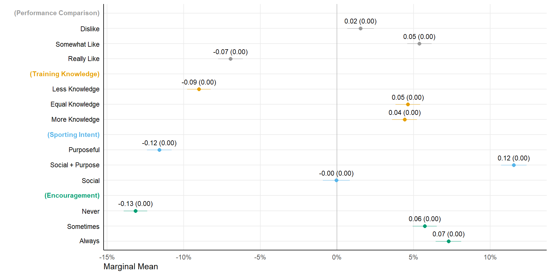
4 AMCEs
In our fully randomized design, average marginal component effects (AMCE) (Hainmueller, Hopkins, and Yamamoto 2014) simply represent differences between marginal means at each feature level and the marginal mean in the reference category, ignoring other features.
amce <- cregg::cj(data, f1, id = ~id)
fshowdf(amce)| outcome | statistic | feature | level | estimate | std.error | z | p | lower | upper |
|---|---|---|---|---|---|---|---|---|---|
| choice | amce | comparison | really likes to compare sports performances | 0.00 | NA | NA | NA | NA | NA |
| choice | amce | comparison | somewhat likes to compare sports performances | 0.12 | 0.01 | 18.54 | 0.00 | 0.11 | 0.14 |
| choice | amce | comparison | does not like to compare sports performances | 0.08 | 0.01 | 11.51 | 0.00 | 0.07 | 0.10 |
| choice | amce | knowledge | knows more than you about effective training and the right technique | 0.00 | NA | NA | NA | NA | NA |
| choice | amce | knowledge | knows as much as you about effective training and the right technique | 0.00 | 0.01 | 0.45 | 0.65 | -0.01 | 0.02 |
| choice | amce | knowledge | knows less than you about effective training and the right technique | -0.13 | 0.01 | -19.40 | 0.00 | -0.14 | -0.12 |
| choice | amce | companionship | exercises to socially engage | 0.00 | NA | NA | NA | NA | NA |
| choice | amce | companionship | wants a combination of social interaction and purposeful training | 0.12 | 0.01 | 15.68 | 0.00 | 0.10 | 0.13 |
| choice | amce | companionship | exercises purposefully and seriously | -0.11 | 0.01 | -15.52 | 0.00 | -0.13 | -0.10 |
| choice | amce | encouragement | always encourages you | 0.00 | NA | NA | NA | NA | NA |
| choice | amce | encouragement | sometimes encourages you | -0.02 | 0.01 | -2.61 | 0.01 | -0.03 | 0.00 |
| choice | amce | encouragement | never encourages you | -0.21 | 0.01 | -29.88 | 0.00 | -0.22 | -0.19 |
# also include coeffients as lables, but leave out the labels for the reference level
amce$showlabel <- ifelse(is.na(amce$std.error), 0, 1)

plot(amce, size = 2) + ftheme() + scale_colour_manual(values = cbPalette) + geom_text(data = subset(amce,
    showlabel == 1), aes(label = sprintf("%0.2f (%0.2f)", estimate, std.error)), size = 3, colour = "black",
    position = position_nudge(y = 0.5)) + scale_y_discrete(labels = rev(newlabels)) + scale_color_manual(labels = c("Performance comparison",
    "Training knowledge", "Sporting intent", "Encouragement"), values = cbPalette) + theme(axis.line = element_line(),
    axis.text.y.left = element_text(color = rev(headcol)), legend.position = "none")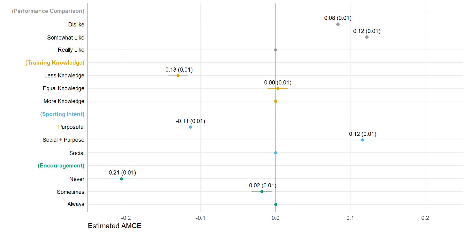
4.1 Reference category diagnostics for AMCEs
4.1.1 Performance comparison
amce_diagnostic1 <- cregg::amce_by_reference(data, choice ~ comparison, variable = ~comparison, id = ~id)
plot1 <- plot(amce_diagnostic1, group = "REFERENCE", legend_title = "Ref. cat.") + ftheme() + scale_colour_manual(values = cbPalette)
plot1 + theme(legend.direction = "vertical")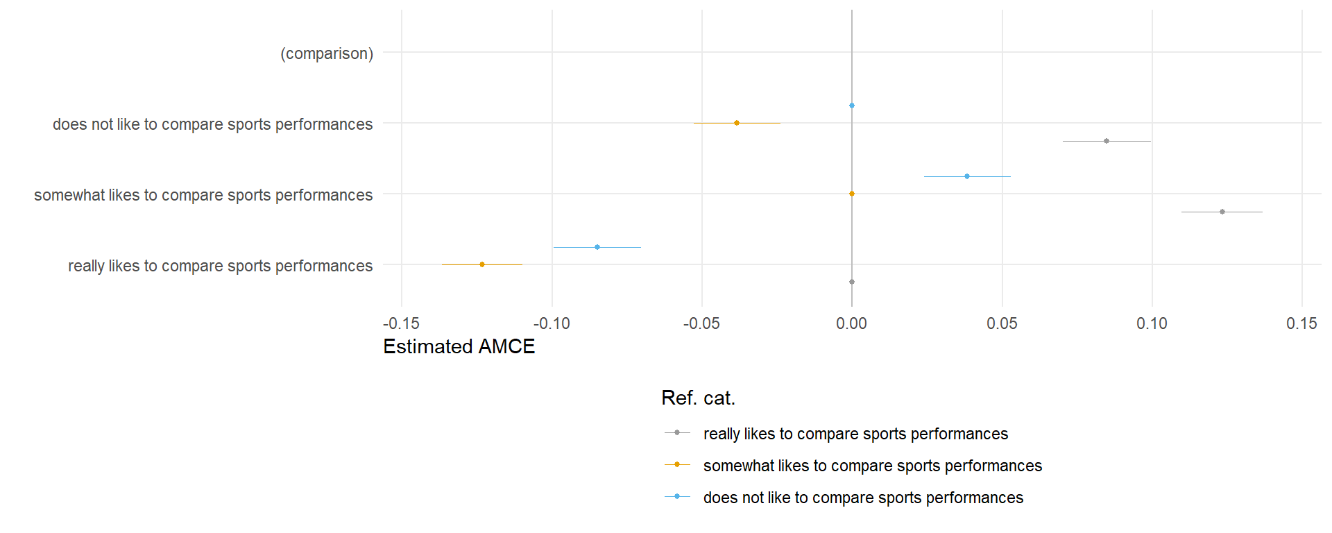
4.1.2 Training knowledge
amce_diagnostic2 <- cregg::amce_by_reference(data, choice ~ knowledge, variable = ~knowledge, id = ~id)
plot2 <- plot(amce_diagnostic2, group = "REFERENCE", legend_title = "Ref. cat.") + ftheme() + scale_colour_manual(values = cbPalette)
plot2 + theme(legend.direction = "vertical")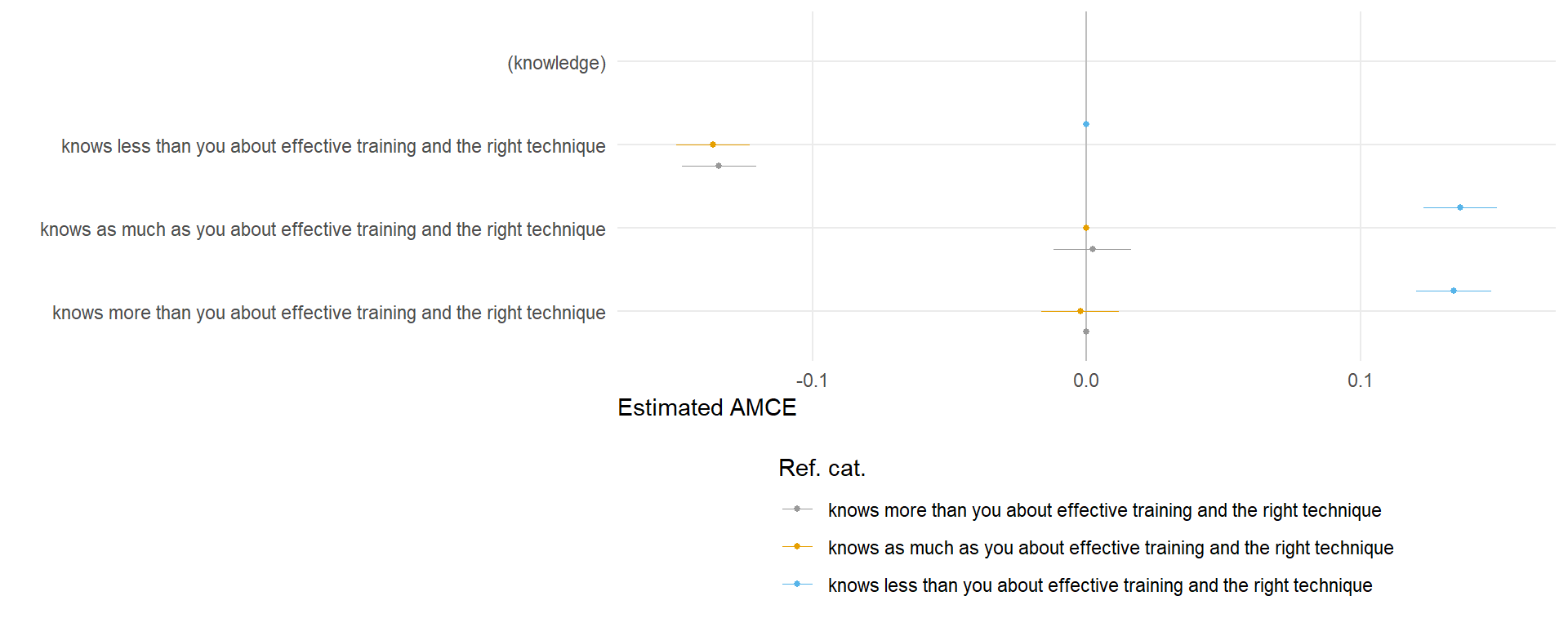
4.1.3 Companionship
amce_diagnostic3 <- cregg::amce_by_reference(data, choice ~ companionship, variable = ~companionship,
    id = ~id)
plot3 <- plot(amce_diagnostic3, group = "REFERENCE", legend_title = "Ref. cat.") + ftheme() + scale_colour_manual(values = cbPalette)
plot3 + theme(legend.direction = "vertical")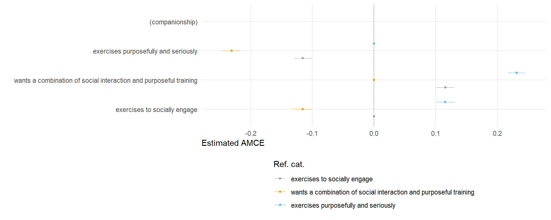
4.1.4 Encouragement
amce_diagnostic4 <- cregg::amce_by_reference(data, choice ~ encouragement, variable = ~encouragement,
    id = ~id)
plot4 <- plot(amce_diagnostic4, group = "REFERENCE", legend_title = "Ref. cat.") + ftheme() + scale_colour_manual(values = cbPalette)
plot4 + theme(legend.direction = "vertical")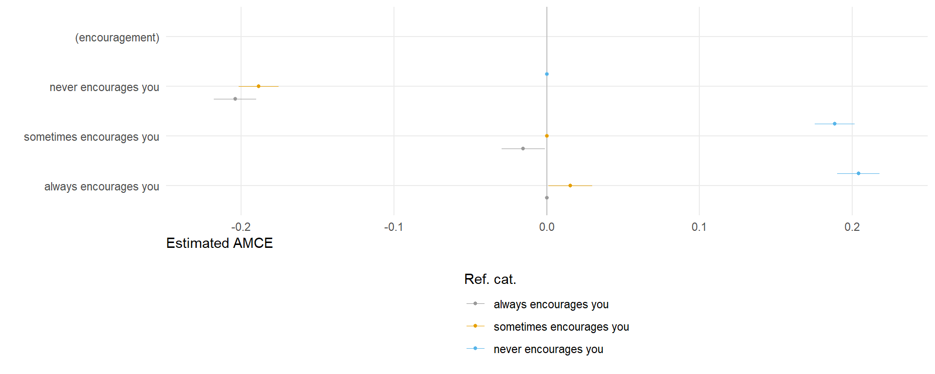
5 Subgroup analysis
5.1 Subgroup marginal means
Estimate conditional marginal means and differences between conditional marginal means to describe differences in preference level between subgroups. To formally test for groups differences in preferences toward particular features, I use omnibus nested model comparisons.
5.1.1 Male vs female
data$Sex <- NA_real_
data$Sex[data$gender == "man"] <- 1L
data$Sex[data$gender == "woman"] <- 2L
data$Sex <- factor(data$Sex, 1:2, c("Male", "Female"))

# conditional MM
mm <- cregg::cj(na.omit(data), f1, id = ~id, estimate = "mm", by = ~Sex)
mm <- mm %>%
    arrange(level, feature)

# substract baseline marginal mean
mm$estimate <- mm$estimate - (1/3)
mm$upper <- mm$upper - (1/3)
mm$lower <- mm$lower - (1/3)

# difference between subgroups
diff_mm <- cregg::cj(data, f1, id = ~id, estimate = "mm_diff", by = ~Sex)

# combine plots
mm <- rbind(mm, diff_mm)
mm$BY <- factor(mm$BY, levels = rev(levels(mm$BY)))
mm$showlabel <- ifelse(is.na(mm$std.error), 0, 1)

# plot with grouping
p1 <- plot(mm, group = "BY", feature_headers = TRUE, size = 1) + ggplot2::facet_wrap(~feature, ncol = 1L,
    scales = "free_y", strip.position = "right") + scale_color_manual(values = c("#56B4E9", "#E69F00",
    "#999999"), breaks = c("Female", "Male", "Female - Male")) + scale_x_continuous(labels = scales::percent) +
    labs(x = "") + ftheme() + theme(strip.text.y = element_blank(), strip.background = element_blank(),
    panel.background = element_rect(color = "darkgrey"), axis.text.y = element_blank(), legend.position = "top",
    legend.direction = "vertical")

# test of preference heterogeneity (nested model comparison test)
cregg::cj_anova(na.omit(data), choice ~ comparison, by = ~Sex)
#> Analysis of Deviance Table
#>
#> Model 1: choice ~ comparison
#> Model 2: choice ~ comparison + Sex + comparison:Sex
#> Resid. Df Resid. Dev Df Deviance F Pr(>F)
#> 1 18528 4073.0
#> 2 18525 4062.7 3 10.263 15.599 3.947e-10 ***
#> ---
#> Signif. codes: 0 '***' 0.001 '**' 0.01 '*' 0.05 '.' 0.1 ' ' 1cregg::cj_anova(na.omit(data), choice ~ knowledge, by = ~Sex)#> Analysis of Deviance Table
#>
#> Model 1: choice ~ knowledge
#> Model 2: choice ~ knowledge + Sex + knowledge:Sex
#> Resid. Df Resid. Dev Df Deviance F Pr(>F)
#> 1 18528 4039.9
#> 2 18525 4039.7 3 0.27112 0.4144 0.7426cregg::cj_anova(na.omit(data), choice ~ companionship, by = ~Sex)#> Analysis of Deviance Table
#>
#> Model 1: choice ~ companionship
#> Model 2: choice ~ companionship + Sex + companionship:Sex
#> Resid. Df Resid. Dev Df Deviance F Pr(>F)
#> 1 18528 3946.1
#> 2 18525 3944.8 3 1.2851 2.0116 0.11cregg::cj_anova(na.omit(data), choice ~ encouragement, by = ~Sex)#> Analysis of Deviance Table
#>
#> Model 1: choice ~ encouragement
#> Model 2: choice ~ encouragement + Sex + encouragement:Sex
#> Resid. Df Resid. Dev Df Deviance F Pr(>F)
#> 1 18528 3922.8
#> 2 18525 3922.1 3 0.76103 1.1982 0.30875.1.2 active vs non-active
data$Active <- NA_real_
data$Active[data$activeW2 == "yes"] <- 2L
data$Active[data$activeW2 == "no"] <- 1L
data$Active <- factor(data$Active, 1:2, c("Inactive", "Active"))

# conditional MM
mm <- cregg::cj(data, f1, id = ~id, estimate = "mm", by = ~Active)
mm <- mm %>%
    arrange(level, feature)

# substract baseline marginal mean
mm$estimate <- mm$estimate - (1/3)
mm$upper <- mm$upper - (1/3)
mm$lower <- mm$lower - (1/3)

# difference between subgroups
diff_mm <- cregg::cj(data, f1, id = ~id, estimate = "mm_diff", by = ~Active)

# combine plots
mm <- rbind(mm, diff_mm)
mm$BY <- factor(mm$BY, levels = rev(levels(mm$BY)))
mm$showlabel <- ifelse(is.na(mm$std.error), 0, 1)

# custom headers/levels
levels(mm$feature) <- c("**Performance Comparison**", "**Training Knowledge**", "**Sporting Intent**",
    "**Encouragement**")
levels(mm$level) <- c("Really Like", "Somewhat Like", "Dislike", "More Knowledge", "Equal Knowledge",
    "Less Knowledge", "Social", "Social + Purpose", "Purposeful", "Always", "Sometimes", "Never")

# plot with grouping
p2 <- plot(mm, group = "BY", feature_headers = TRUE, size = 1) + ggplot2::facet_wrap(~feature, ncol = 1L,
    scales = "free_y", strip.position = "right") + scale_x_continuous(labels = scales::percent) + scale_color_manual(values = c("#56B4E9",
    "#E69F00", "#999999"), breaks = c("Active", "Inactive", "Active - Inactive")) + labs(x = "") + ftheme() +
    theme(strip.text.y = element_blank(), strip.background = element_blank(), panel.background = element_rect(color = "darkgrey"),
        axis.text.y = element_markdown(), legend.position = "top", legend.direction = "vertical")

# test of preference heterogeneity (nested model comparison test)
cregg::cj_anova(data, choice ~ comparison, by = ~Active)
#> Analysis of Deviance Table
#>
#> Model 1: choice ~ comparison
#> Model 2: choice ~ comparison + Active + comparison:Active
#> Resid. Df Resid. Dev Df Deviance F Pr(>F)
#> 1 28851 6335.0
#> 2 28848 6331.4 3 3.5963 5.462 0.000947 ***
#> ---
#> Signif. codes: 0 '***' 0.001 '**' 0.01 '*' 0.05 '.' 0.1 ' ' 1cregg::cj_anova(data, choice ~ knowledge, by = ~Active)#> Analysis of Deviance Table
#>
#> Model 1: choice ~ knowledge
#> Model 2: choice ~ knowledge + Active + knowledge:Active
#> Resid. Df Resid. Dev Df Deviance F Pr(>F)
#> 1 28851 6294.6
#> 2 28848 6294.2 3 0.41914 0.6403 0.589cregg::cj_anova(data, choice ~ companionship, by = ~Active)#> Analysis of Deviance Table
#>
#> Model 1: choice ~ companionship
#> Model 2: choice ~ companionship + Active + companionship:Active
#> Resid. Df Resid. Dev Df Deviance F Pr(>F)
#> 1 28851 6155.0
#> 2 28848 6130.3 3 24.64 38.65 < 2.2e-16 ***
#> ---
#> Signif. codes: 0 '***' 0.001 '**' 0.01 '*' 0.05 '.' 0.1 ' ' 1cregg::cj_anova(data, choice ~ encouragement, by = ~Active)#> Analysis of Deviance Table
#>
#> Model 1: choice ~ encouragement
#> Model 2: choice ~ encouragement + Active + encouragement:Active
#> Resid. Df Resid. Dev Df Deviance F Pr(>F)
#> 1 28851 6164.8
#> 2 28848 6159.7 3 5.1754 8.0794 2.238e-05 ***
#> ---
#> Signif. codes: 0 '***' 0.001 '**' 0.01 '*' 0.05 '.' 0.1 ' ' 15.1.3 High vs low frequency
# sports_frequency <- ifelse(is.na(data$sportsfreq), 0, as.numeric(data$sportsfreq))
# hist(sports_frequency) ftable(psych::describe(sports_frequency))

# here, focus only on those currently active..
data$Frequency <- NA_real_
data$Frequency[data$sportsfreq < 3] <- 1L
data$Frequency[data$sportsfreq >= 3] <- 2L
data$Frequency <- factor(data$Frequency, 1:2, c("Low", "High"))

# conditional MM
mm <- cregg::cj(data, f1, id = ~id, estimate = "mm", by = ~Frequency)
mm <- mm %>%
    arrange(level, feature)

# substract baseline marginal mean
mm$estimate <- mm$estimate - (1/3)
mm$upper <- mm$upper - (1/3)
mm$lower <- mm$lower - (1/3)

# difference between subgroups
diff_mm <- cregg::cj(data, f1, id = ~id, estimate = "mm_diff", by = ~Frequency)

# combine plots
mm <- rbind(mm, diff_mm)
mm$BY <- factor(mm$BY, levels = rev(levels(mm$BY)))
mm$showlabel <- ifelse(is.na(mm$std.error), 0, 1)

# plot with grouping
p3 <- plot(mm, group = "BY", feature_headers = TRUE, size = 1) + ggplot2::facet_wrap(~feature, ncol = 1L,
    scales = "free_y", strip.position = "right") + scale_color_manual(values = c("#56B4E9", "#E69F00",
    "#999999"), breaks = c("High", "Low", "High - Low")) + scale_x_continuous(labels = scales::percent) +
    ftheme() + theme(strip.text.y = element_blank(), strip.background = element_blank(), panel.background = element_rect(color = "darkgrey"),
    axis.text.y = element_blank(), legend.position = "top", legend.direction = "vertical")

# test of preference heterogeneity (nested model comparison test)
cregg::cj_anova(data[!is.na(data$Frequency), ], choice ~ comparison, by = ~Frequency)
#> Analysis of Deviance Table
#>
#> Model 1: choice ~ comparison
#> Model 2: choice ~ comparison + Frequency + comparison:Frequency
#> Resid. Df Resid. Dev Df Deviance F Pr(>F)
#> 1 18600 4088.3
#> 2 18597 4086.7 3 1.6084 2.4397 0.06243 .
#> ---
#> Signif. codes: 0 '***' 0.001 '**' 0.01 '*' 0.05 '.' 0.1 ' ' 1cregg::cj_anova(data[!is.na(data$Frequency), ], choice ~ knowledge, by = ~Frequency)#> Analysis of Deviance Table
#>
#> Model 1: choice ~ knowledge
#> Model 2: choice ~ knowledge + Frequency + knowledge:Frequency
#> Resid. Df Resid. Dev Df Deviance F Pr(>F)
#> 1 18600 4056.1
#> 2 18597 4053.8 3 2.2615 3.4582 0.01565 *
#> ---
#> Signif. codes: 0 '***' 0.001 '**' 0.01 '*' 0.05 '.' 0.1 ' ' 1cregg::cj_anova(data[!is.na(data$Frequency), ], choice ~ companionship, by = ~Frequency)#> Analysis of Deviance Table
#>
#> Model 1: choice ~ companionship
#> Model 2: choice ~ companionship + Frequency + companionship:Frequency
#> Resid. Df Resid. Dev Df Deviance F Pr(>F)
#> 1 18600 3961.6
#> 2 18597 3949.7 3 11.886 18.656 4.446e-12 ***
#> ---
#> Signif. codes: 0 '***' 0.001 '**' 0.01 '*' 0.05 '.' 0.1 ' ' 1cregg::cj_anova(data[!is.na(data$Frequency), ], choice ~ encouragement, by = ~Frequency)#> Analysis of Deviance Table
#>
#> Model 1: choice ~ encouragement
#> Model 2: choice ~ encouragement + Frequency + encouragement:Frequency
#> Resid. Df Resid. Dev Df Deviance F Pr(>F)
#> 1 18600 3938.9
#> 2 18597 3938.8 3 0.10924 0.1719 0.91545.1.3.1 different cut-off high/low
high (> 3) vs. low (≤ 3)
# sports_frequency <- ifelse(is.na(data$sportsfreq), 0, as.numeric(data$sportsfreq))
# hist(sports_frequency) ftable(psych::describe(sports_frequency))

# here, focus only on those currently active..
data$Frequency <- NA_real_
data$Frequency[data$sportsfreq < 4] <- 1L
data$Frequency[data$sportsfreq > 3] <- 2L
data$Frequency <- factor(data$Frequency, 1:2, c("Low", "High"))

# prop.table(table(data$Frequency)) #63 vs 37

# conditional MM
mm <- cregg::cj(data, f1, id = ~id, estimate = "mm", by = ~Frequency)
mm <- mm %>%
    arrange(level, feature)

# substract baseline marginal mean
mm$estimate <- mm$estimate - (1/3)
mm$upper <- mm$upper - (1/3)
mm$lower <- mm$lower - (1/3)

# difference between subgroups
diff_mm <- cregg::cj(data, f1, id = ~id, estimate = "mm_diff", by = ~Frequency)

# combine plots
mm <- rbind(mm, diff_mm)
mm$BY <- factor(mm$BY, levels = rev(levels(mm$BY)))
mm$showlabel <- ifelse(is.na(mm$std.error), 0, 1)

# custom headers/levels
levels(mm$feature) <- c("**Performance Comparison**", "**Training Knowledge**", "**Sporting Intent**",
    "**Encouragement**")
levels(mm$level) <- c("Really Like", "Somewhat Like", "Dislike", "More Knowledge", "Equal Knowledge",
    "Less Knowledge", "Social", "Social + Purpose", "Purposeful", "Always", "Sometimes", "Never")

# plot with grouping
p4 <- plot(mm, group = "BY", feature_headers = TRUE, size = 1) + ggplot2::facet_wrap(~feature, ncol = 1L,
    scales = "free_y", strip.position = "right") + scale_x_continuous(labels = scales::percent) + scale_color_manual(values = c("#56B4E9",
    "#E69F00", "#999999"), breaks = c("High", "Low", "High - Low")) + labs(x = "") + ftheme() + theme(strip.text.y = element_blank(),
    strip.background = element_blank(), panel.background = element_rect(color = "darkgrey"), axis.text.y = element_markdown(),
    legend.position = "top", legend.direction = "vertical")

# test of preference heterogeneity (nested model comparison test)
# cregg::cj_anova(data[!is.na(data$Frequency),], choice ~ comparison, by = ~Frequency)
# cregg::cj_anova(data[!is.na(data$Frequency),], choice ~ knowledge, by = ~Frequency)
# cregg::cj_anova(data[!is.na(data$Frequency),], choice ~ companionship, by = ~Frequency)
# cregg::cj_anova(data[!is.na(data$Frequency),], choice ~ encouragement, by = ~Frequency)

print(p4)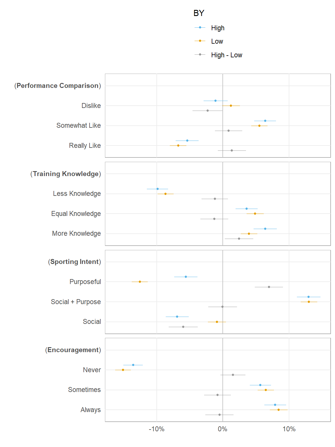
5.2 Plot
(multiplot <- ggpubr::ggarrange(p2, p3, p1, ncol = 3, nrow = 1, widths = c(1.9, 1, 1)))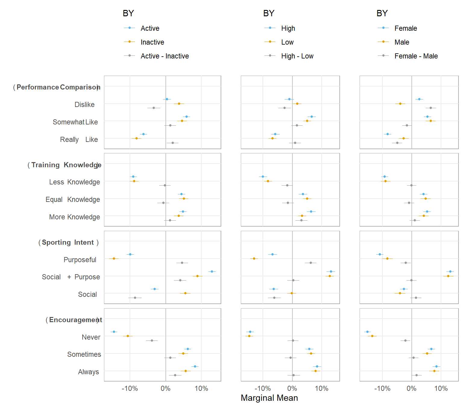
# ggsave('./figures/cmms.pneg', multiplot)6 Diagnostics
6.1 Frequencies
Of conjoint features (to ensure equal display frequency):
plot(cregg::cj_freqs(data, choice ~ comparison + knowledge + companionship + encouragement + Sex + Active +
    Frequency, id = ~id)) + ftheme() + scale_colour_manual(values = cbPalette)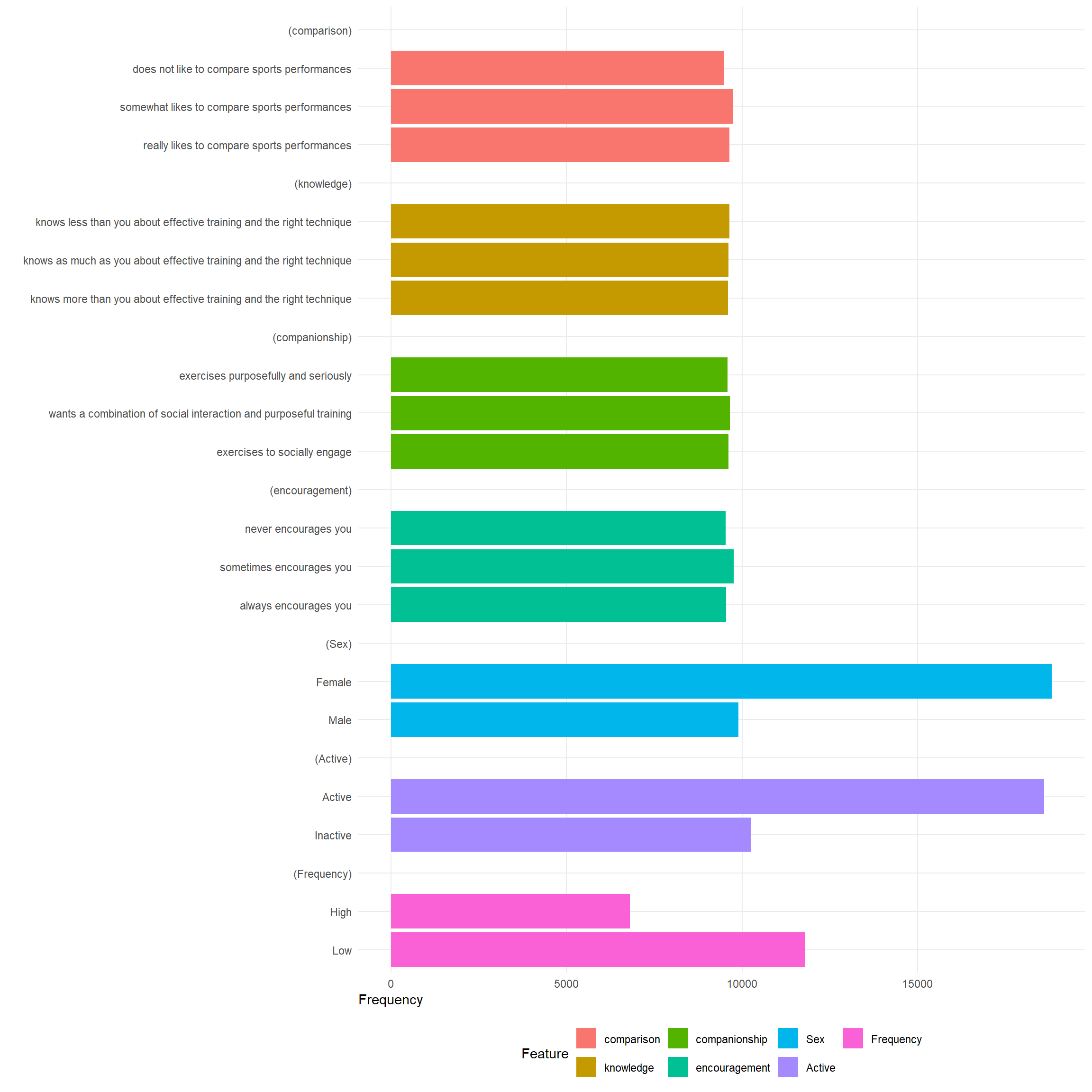
References
Copyright © Rob Franken