Analysis
Last compiled on augustus, 2024
1 Getting started
To copy the code, click the button in the upper right corner of the code-chunks.
1.1 clean up
rm(list = ls())
gc()
1.2 general custom functions
fpackage.check: Check if packages are installed (and install if not) in Rfsave: Function to save data with time stamp in correct directoryfload: Function to load R-objects under new namesftheme: pretty ggplot2 themefshowdf: Print objects (tibble/data.frame) nicely on screen in.Rmd.ffit: fit a series of (here, generalized linear mixed-effects) models
fpackage.check <- function(packages) {
    lapply(packages, FUN = function(x) {
        if (!require(x, character.only = TRUE)) {
            install.packages(x, dependencies = TRUE)
            library(x, character.only = TRUE)
        }
    })
}

fsave <- function(x, file, location = "./data/processed/", ...) {
    if (!dir.exists(location))
        dir.create(location)
    datename <- substr(gsub("[:-]", "", Sys.time()), 1, 8)
    totalname <- paste(location, datename, file, sep = "")
    print(paste("SAVED: ", totalname, sep = ""))
    save(x, file = totalname)
}

fload <- function(fileName) {
    load(fileName)
    get(ls()[ls() != "fileName"])
}

# extrafont::font_import(paths = c('C:/Users/u244147/Downloads/Jost/', prompt = FALSE))
ftheme <- function() {

    # download font at https://fonts.google.com/specimen/Jost/
    theme_minimal(base_family = "Jost") + theme(panel.grid.minor = element_blank(), plot.title = element_text(family = "Jost",
        face = "bold"), axis.title = element_text(family = "Jost Medium"), axis.title.x = element_text(hjust = 0),
        axis.title.y = element_text(hjust = 1), strip.text = element_text(family = "Jost", face = "bold",
            size = rel(0.75), hjust = 0), strip.background = element_rect(fill = "grey90", color = NA),
        legend.position = "bottom")
}

fshowdf <- function(x, digits = 2, ...) {
    knitr::kable(x, digits = digits, "html", ...) %>%
        kableExtra::kable_styling(bootstrap_options = c("striped", "hover")) %>%
        kableExtra::scroll_box(width = "100%", height = "300px")
}

ffit <- function(formula, data) {
    tryCatch({
        model <- lme4::glmer(formula, data = data, family = binomial(link = "logit"), control = glmerControl(optimizer = "bobyqa",
            optCtrl = list(maxfun = 1e+05)))
        cat("Fitting model:", as.character(formula), "\n")
        summary(model)
        cat("\n")
        return(model)
    }, error = function(e) {
        cat("Error fitting model:", as.character(formula), "\n")
        cat("Error message:", conditionMessage(e), "\n")
        return(NULL)
    })
}
1.3 necessary packages
tidyverselme4: fitting random effects modelslmtest: diagnostics test (likelihood ratio test)car: companion applied regression (calculate VIF)texreg: output to HTML tableggplot2ggpubr: format ggplot2 plotsggh4x: hacks for ggplot2ggtext: text renderingparallel: parallel computing
packages = c("tidyverse", "lme4", "lmtest", "car", "texreg", "ggplot2", "ggpubr", "ggh4x", "ggtext",
    "parallel")
fpackage.check(packages)
rm(packages)
1.4 load data-set
Load the replicated data-set. To load these file, adjust the filename
in the following code so that it matches the most recent version of the
.RDa file you have in your ./data/processed/
folder.
You may also obtain them by downloading: Download networkdata.Rda
# list files in processed data folder
list.files("./data/processed/")

# get todays date:
today <- gsub("-", "", Sys.Date())

# use fload
df <- fload(paste0("./data/processed/", today, "networkdata.Rda"))
1.5 last alterations
- subset sports partners at t to study tie maintenance at t+1
- binary outcome (sports partner: yes/no; 1/0)
- calculate no. of ‘replacement candidates’ (i.e., no. of other sports partners, other than alter j, with whom ego does the sport type he/she does with alter)
- proximity levels
- sports settings
- dyadic skill category combinations (HH, HM, HL, ML, MM, LL)
- also difference score in skill
- alter sports frequency and ego/alter mean
- gender composition dyad (MM, FM, FF)
- type of sport (fitness, endurance, team, miscellaneous)
#subset sports partners at t
df <- df[df$csn == 1,]

#outcome
df$y <- ifelse(df$Ycsn == 1, 1, 0)

#calculate rpelacement candidates: no. of other sports partners next to alter j, at time t, with whom ego does the same activity type
df$nreplace <- NA

for (i in unique(df$ego)) {
  for (t in unique(df$period[df$ego == i])) {
    for (j in unique(df$alterid[df$ego == i & df$period == t])) {

      #get activity type alter j does with ego at t
      activity <- df$sporttogether[df$ego == i & df$alterid == j & df$period == t]

      #get number of *other* alters with whom ego does the same activity at t (ie, replacement candidates)
      df$nreplace[df$ego == i & df$alterid == j & df$period == t] <- length(which(df$sporttogether[df$ego == i & !df$alterid == j & df$period == t] == activity))
    }
  }
}

df$proximity <- factor(df$proximity, levels = c("far","close","roommate"))
df$close <- ifelse(df$proximity == "close",1,0)
df$roommate <- ifelse(df$proximity == "roommate",1,0)
df$far <- ifelse(df$proximity == "far",1,0)

df$ego_context[is.na(df$ego_context)] <- "missing"
df$ego_context <- factor(df$ego_context, levels = c("club", "informal", "gym", "alone", "missing"))
df$club <- ifelse(df$ego_context == "club",1,0)
df$informal <- ifelse(df$ego_context == "informal",1,0)
df$gym <- ifelse(df$ego_context == "gym",1,0)
df$alone <- ifelse(df$ego_context == "alone",1,0)
df$missing <- ifelse(df$ego_context == "missing",1,0)

df$HH <- ifelse(df$ego_grade > 7 & df$alter_grade > 7, 1, 0)
df$HM <- ifelse( ((df$ego_grade > 7 & df$alter_grade > 5 & df$alter_grade < 8) | (df$alter_grade > 7 & df$ego_grade > 5 & df$ego_grade < 8)), 1, 0)
df$HL <- ifelse( ((df$ego_grade > 7 & df$alter_grade < 6) | (df$alter_grade > 7 & df$ego_grade < 6)), 1, 0)
df$MM <- ifelse( ((df$ego_grade > 5 & df$ego_grade < 8 & df$alter_grade > 5 & df$alter_grade < 8)), 1, 0)
df$ML <- ifelse( ((df$ego_grade > 5 & df$ego_grade < 8 & df$alter_grade < 6) | (df$ego_grade < 6 & df$alter_grade < 8 & df$alter_grade > 5)), 1, 0)
df$LL <- ifelse( ((df$ego_grade < 6 & df$alter_grade < 6)), 1, 0)

df$skills <- factor(
  1 * (((df$ego_grade > 5 & df$ego_grade < 8 & df$alter_grade > 5 & df$alter_grade < 8))) +  # MM
  2 * (df$ego_grade > 7 & df$alter_grade > 7) +        # HH
  3 * (((df$ego_grade > 7 & df$alter_grade > 5 & df$alter_grade < 8) | (df$alter_grade > 7 & df$ego_grade > 5 & df$ego_grade < 8))) +  # HM
  4 * (((df$ego_grade > 7 & df$alter_grade < 6) | (df$alter_grade > 7 & df$ego_grade < 6))) +  # HL
  5 * (((df$ego_grade > 5 & df$ego_grade < 8 & df$alter_grade < 6) | (df$ego_grade < 6 & df$alter_grade < 8 & df$alter_grade > 5))) +  # ML
  6 * (((df$ego_grade < 6 & df$alter_grade < 6))),        # LL
  levels = c(1, 2, 3, 4, 5, 6),
  labels = c("MM", "HH", "HM", "HL", "ML", "LL")
)

df$dif_skill <- abs(df$ego_grade - df$alter_grade)

df$alter_freq2 <- ifelse(df$alter_freq == "1 keer per week", 1,
                        ifelse(df$alter_freq == "2 of 3 keer per week", 2.5,
                             ifelse(df$alter_freq == "4 of 5 keer per week", 4.5,
                                    ifelse(df$alter_freq == "6 keer per week of vaker", 6.5,
                                           ifelse(df$alter_freq == "Minder dan 1 keer per maand", 0.125,
                                                  ifelse(df$alter_freq == "1 of 2 keer per maand", 0.375,
                                                         ifelse(df$alter_freq == "1 of 2 keer per maand", 0.375, NA)))))))
df$ego_freq <- as.numeric(df$ego_freq)
df$ego_activew1 <- ifelse(df$ego_meanfreq >0, 1, 0)

df <- df %>%
  mutate(mean_freq = rowMeans(select(., alter_freq2, ego_freq), na.rm = TRUE))

#df$ego_meanskill[is.na(df$ego_meanskill)] <- mean(df$ego_meanskill[which(!duplicated(df$ego))], na.rm=TRUE )

df$alter_age <- as.numeric(df$alter_age)

df$ff <- ifelse(df$ego_female == 1 & df$alter_female == 1, 1, 0)
df$fm <- ifelse( ((df$ego_female == 1 & df$alter_female == 0) | (df$ego_female == 0 & df$alter_female == 1)), 1, 0)
df$mm <- ifelse(df$ego_female == 0 & df$alter_female == 0, 1, 0)

df$gender <- factor(
  1 * (df$ego_female == 0 & df$alter_female == 0) +  # MM
  2 * ((df$ego_female == 1 & df$alter_female == 0) | (df$ego_female == 0 & df$alter_female == 1)) +  # FM
  3 * (df$ego_female == 1 & df$alter_female == 1),  # FF
  levels = c(1, 2, 3),
  labels = c("MM", "FM", "FF")
)

df$ego_quit[is.na(df$ego_quit)] <- 0

#exclude kin
df[df$kin == "0",] -> df

#types of sport
df$fitness <- ifelse(df$sporttogether == 1,1,0)
df$endurance <- ifelse(df$sporttogether %in% c(2,5,7), 1, 0)
df$team <- ifelse(df$sporttogether %in% c(3,10,12), 1, 0)
df$misc <- ifelse(!df$sporttogether %in% c(1,2,5,7,3,10,12),1,0)

df$sporttype <- factor(
  1 * (df$fitness == 1) +
  2 * (df$endurance == 1) +
  3 * (df$team == 1) +
  4 * (df$misc == 1),
  levels = c(1:4),
  labels = c("fitness", "endurance", "team", "miscellaneous")
)
2 Descriptives
# listwise deletion
df %>%
    select(proximity, roommate, close, far, frequency.t, closeness.t, duration, csn, bff, study, cdn,
        gender, mm, fm, ff, period, y, ego, alterid, ego_activew1, mean_freq, skills, HH, HM, HL, MM,
        ML, LL, ego_grade, dif_skill, ego_context, club, informal, gym, alone, missing, sporttogether,
        nreplace, sporttype, fitness, endurance, team, misc) %>%
    filter(complete.cases(.)) -> df

# describe
df %>%
    select(-c(proximity, gender, skills, ego_context, ego, alterid, ego_activew1, sporttogether, sporttype)) %>%
    psych::describe() %>%
fshowdf(caption = "descriptive statistics of ego's (non-kin) social relations WITHIN SPORTS at time t")| vars | n | mean | sd | median | trimmed | mad | min | max | range | skew | kurtosis | se | |
|---|---|---|---|---|---|---|---|---|---|---|---|---|---|
| roommate | 1 | 1426 | 0.12 | 0.33 | 0 | 0.03 | 0.00 | 0.00 | 1.00 | 1.00 | 2.29 | 3.23 | 0.01 |
| close | 2 | 1426 | 0.70 | 0.46 | 1 | 0.75 | 0.00 | 0.00 | 1.00 | 1.00 | -0.87 | -1.25 | 0.01 |
| far | 3 | 1426 | 0.18 | 0.38 | 0 | 0.10 | 0.00 | 0.00 | 1.00 | 1.00 | 1.69 | 0.85 | 0.01 |
| frequency.t | 4 | 1426 | 6.04 | 1.04 | 6 | 6.20 | 1.48 | 1.00 | 7.00 | 6.00 | -1.78 | 4.87 | 0.03 |
| closeness.t | 5 | 1426 | 3.00 | 0.93 | 3 | 3.09 | 1.48 | 1.00 | 4.00 | 3.00 | -0.52 | -0.74 | 0.02 |
| duration | 6 | 1426 | 3.91 | 3.95 | 2 | 3.25 | 2.97 | 0.00 | 15.00 | 15.00 | 1.31 | 0.95 | 0.10 |
| csn | 7 | 1426 | 1.00 | 0.00 | 1 | 1.00 | 0.00 | 1.00 | 1.00 | 0.00 | NaN | NaN | 0.00 |
| bff | 8 | 1426 | 0.41 | 0.49 | 0 | 0.39 | 0.00 | 0.00 | 1.00 | 1.00 | 0.35 | -1.88 | 0.01 |
| study | 9 | 1426 | 0.16 | 0.37 | 0 | 0.08 | 0.00 | 0.00 | 1.00 | 1.00 | 1.81 | 1.28 | 0.01 |
| cdn | 10 | 1426 | 0.33 | 0.47 | 0 | 0.29 | 0.00 | 0.00 | 1.00 | 1.00 | 0.70 | -1.51 | 0.01 |
| mm | 11 | 1426 | 0.15 | 0.36 | 0 | 0.07 | 0.00 | 0.00 | 1.00 | 1.00 | 1.93 | 1.74 | 0.01 |
| fm | 12 | 1426 | 0.27 | 0.44 | 0 | 0.21 | 0.00 | 0.00 | 1.00 | 1.00 | 1.06 | -0.88 | 0.01 |
| ff | 13 | 1426 | 0.58 | 0.49 | 1 | 0.60 | 0.00 | 0.00 | 1.00 | 1.00 | -0.33 | -1.89 | 0.01 |
| period | 14 | 1426 | 1.33 | 0.47 | 1 | 1.28 | 0.00 | 1.00 | 2.00 | 1.00 | 0.73 | -1.46 | 0.01 |
| y | 15 | 1426 | 0.43 | 0.50 | 0 | 0.41 | 0.00 | 0.00 | 1.00 | 1.00 | 0.28 | -1.92 | 0.01 |
| mean_freq | 16 | 1426 | 2.04 | 1.34 | 2 | 1.91 | 1.48 | 0.12 | 6.75 | 6.62 | 0.84 | 0.62 | 0.04 |
| HH | 17 | 1426 | 0.21 | 0.41 | 0 | 0.14 | 0.00 | 0.00 | 1.00 | 1.00 | 1.42 | 0.03 | 0.01 |
| HM | 18 | 1426 | 0.35 | 0.48 | 0 | 0.31 | 0.00 | 0.00 | 1.00 | 1.00 | 0.62 | -1.61 | 0.01 |
| HL | 19 | 1426 | 0.05 | 0.23 | 0 | 0.00 | 0.00 | 0.00 | 1.00 | 1.00 | 3.91 | 13.32 | 0.01 |
| MM | 20 | 1426 | 0.24 | 0.43 | 0 | 0.18 | 0.00 | 0.00 | 1.00 | 1.00 | 1.20 | -0.55 | 0.01 |
| ML | 21 | 1426 | 0.11 | 0.31 | 0 | 0.01 | 0.00 | 0.00 | 1.00 | 1.00 | 2.50 | 4.25 | 0.01 |
| LL | 22 | 1426 | 0.03 | 0.18 | 0 | 0.00 | 0.00 | 0.00 | 1.00 | 1.00 | 5.23 | 25.33 | 0.00 |
| ego_grade | 23 | 1426 | 6.80 | 1.45 | 7 | 6.95 | 1.48 | 1.00 | 10.00 | 9.00 | -0.97 | 1.21 | 0.04 |
| dif_skill | 24 | 1426 | 1.25 | 1.18 | 1 | 1.09 | 1.48 | 0.00 | 9.00 | 9.00 | 1.55 | 4.74 | 0.03 |
| club | 25 | 1426 | 0.35 | 0.48 | 0 | 0.31 | 0.00 | 0.00 | 1.00 | 1.00 | 0.64 | -1.59 | 0.01 |
| informal | 26 | 1426 | 0.12 | 0.32 | 0 | 0.02 | 0.00 | 0.00 | 1.00 | 1.00 | 2.36 | 3.56 | 0.01 |
| gym | 27 | 1426 | 0.25 | 0.43 | 0 | 0.18 | 0.00 | 0.00 | 1.00 | 1.00 | 1.18 | -0.61 | 0.01 |
| alone | 28 | 1426 | 0.10 | 0.31 | 0 | 0.01 | 0.00 | 0.00 | 1.00 | 1.00 | 2.58 | 4.68 | 0.01 |
| missing | 29 | 1426 | 0.18 | 0.39 | 0 | 0.11 | 0.00 | 0.00 | 1.00 | 1.00 | 1.63 | 0.64 | 0.01 |
| nreplace | 30 | 1426 | 1.37 | 1.37 | 1 | 1.21 | 1.48 | 0.00 | 6.00 | 6.00 | 0.70 | -0.54 | 0.04 |
| fitness | 31 | 1426 | 0.27 | 0.44 | 0 | 0.21 | 0.00 | 0.00 | 1.00 | 1.00 | 1.03 | -0.95 | 0.01 |
| endurance | 32 | 1426 | 0.11 | 0.32 | 0 | 0.02 | 0.00 | 0.00 | 1.00 | 1.00 | 2.43 | 3.92 | 0.01 |
| team | 33 | 1426 | 0.16 | 0.36 | 0 | 0.07 | 0.00 | 0.00 | 1.00 | 1.00 | 1.88 | 1.55 | 0.01 |
| misc | 34 | 1426 | 0.46 | 0.50 | 0 | 0.45 | 0.00 | 0.00 | 1.00 | 1.00 | 0.17 | -1.97 | 0.01 |
length(unique(paste0(df$ego, "X", df$alterid))) #N_alter =1222#> [1] 1222nrow(df) #N_observation = 1426#> [1] 14263 Multivariate analyses
3.1 logistic regression
#tie continuation:

formula <- list(
  #model 1: main predictors
  y ~ 1 + (1 | ego) + scale(ego_grade) + scale(dif_skill) + scale(closeness.t) + ego_context + as.factor(period),

  #model 2: control for sports behavior dyad
  y ~ 1 + (1 | ego) + scale(ego_grade) + scale(dif_skill) + scale(closeness.t) + ego_context + as.factor(period) + scale(mean_freq),

  #model 3: include "traditional" dyadic controls
  y ~ 1 + (1 | ego) + scale(ego_grade) + scale(dif_skill) + scale(closeness.t) + ego_context + as.factor(period) + scale(mean_freq) + proximity + scale(frequency.t) + scale(duration) + gender,

  #model 4: add other relational dimensions (multiplexity)
  y ~ 1 + (1 | ego) + scale(ego_grade) + scale(dif_skill)  + scale(closeness.t) + ego_context + as.factor(period) + scale(mean_freq) + proximity + scale(frequency.t) + scale(duration) + gender + bff + cdn + study,

  #model 5: add replacement candidates
  y ~ 1 + (1 | ego) + scale(ego_grade) + scale(dif_skill) + scale(closeness.t) + ego_context + as.factor(period) + scale(mean_freq) + proximity + scale(frequency.t) + scale(duration) + gender + bff + cdn + study + scale(nreplace)
  )

ans <- lapply(formula, ffit, data = df)
lapply(ans, summary)
do.call(lmtest::lrtest,ans)
3.2 output
| M1: main predictors | M2: sports beh. dyad | M3: dyadic covars | M4: multiplexity | M5: replacement candidates | |
|---|---|---|---|---|---|
| (Intercept) | -0.65 (0.12)*** | -0.68 (0.12)*** | -0.80 (0.24)** | -0.93 (0.26)*** | -0.86 (0.26)*** |
| Ego skill | 0.09 (0.07) | 0.01 (0.08) | -0.00 (0.08) | -0.00 (0.08) | 0.00 (0.08) |
| Ego-alter skill diference | -0.08 (0.07) | -0.09 (0.07) | -0.09 (0.07) | -0.10 (0.07) | -0.09 (0.07) |
| Emotional closeness | 0.55 (0.07)*** | 0.56 (0.07)*** | 0.33 (0.09)*** | 0.23 (0.10)* | 0.24 (0.10)* |
| Informal group | -0.22 (0.22) | -0.10 (0.22) | -0.19 (0.23) | -0.25 (0.24) | -0.33 (0.24) |
| Commercial gym | 0.47 (0.17)** | 0.47 (0.17)** | 0.30 (0.18) | 0.27 (0.19) | 0.20 (0.19) |
| Unorganized | 0.13 (0.22) | 0.23 (0.23) | 0.07 (0.24) | 0.05 (0.24) | -0.05 (0.25) |
| Missing | 0.03 (0.24) | 0.06 (0.24) | -0.10 (0.25) | 0.00 (0.25) | 0.01 (0.25) |
| Period: waves 2-3 | 0.68 (0.18)*** | 0.68 (0.18)*** | 0.66 (0.18)*** | 0.61 (0.19)*** | 0.59 (0.19)** |
| Mean sports frequency dyad | 0.21 (0.07)** | 0.16 (0.07)* | 0.16 (0.08)* | 0.18 (0.08)* | |
| Same municipality | 0.36 (0.18)* | 0.39 (0.18)* | 0.39 (0.18)* | ||
| Roommate | 0.19 (0.25) | 0.20 (0.25) | 0.17 (0.25) | ||
| Communication frequency | 0.54 (0.10)*** | 0.50 (0.10)*** | 0.50 (0.10)*** | ||
| Years known | -0.04 (0.07) | -0.07 (0.07) | -0.07 (0.07) | ||
| Woman-man | -0.07 (0.22) | -0.12 (0.22) | -0.13 (0.22) | ||
| Woman-woman | -0.13 (0.20) | -0.15 (0.20) | -0.15 (0.20) | ||
| Friendship | 0.03 (0.18) | 0.01 (0.18) | |||
| Confidant | 0.49 (0.18)** | 0.48 (0.18)** | |||
| Study partner | -0.21 (0.18) | -0.23 (0.18) | |||
| No. of replacement candidates | -0.14 (0.08) | ||||
| AIC | 1830.18 | 1823.41 | 1790.83 | 1786.93 | 1785.89 |
| BIC | 1882.80 | 1881.30 | 1880.30 | 1892.18 | 1896.40 |
| Log Likelihood | -905.09 | -900.71 | -878.42 | -873.47 | -871.94 |
| Num. obs. | 1426 | 1426 | 1426 | 1426 | 1426 |
| Num. groups: ego | 409 | 409 | 409 | 409 | 409 |
| Var: ego (Intercept) | 0.29 | 0.29 | 0.35 | 0.37 | 0.36 |
| ***p < 0.001; **p < 0.01; *p < 0.05 | |||||
3.3 robustness checks
3.3.1 patterns depend on type of sport?
We compare results in sports partnerships in vs. outside fitness.
df %>%
    select(sporttogether) %>%
    table(.) %>%
    prop.table(.)

# of all sports partner observations: 27% are in fitness; this is the most popular sports in dyads
# 11% are in endurance sports (i.e., running, cycling, swimming) 15% are in team (ball) sports
# (i.e., football, hockey, volleybal)

# 1. solution for fitness partners:
ans_fitness <- lapply(formula, ffit, data = df[df$sporttogether == 1, ])
lapply(ans_fitness, summary)

# 2. solution excluding fitness partners:
ans_nfitness <- lapply(formula, ffit, data = df[!df$sporttogether == 1, ])
lapply(ans_nfitness, summary)

# 3. solution for endurance sports partners:
ans_endurance <- lapply(formula, ffit, data = df[df$sporttogether %in% c(2, 5, 7), ])
lapply(ans_endurance, summary)

# 4. solution for team (ball) sports partners:
ans_team <- lapply(formula, ffit, data = df[df$sporttogether %in% c(3, 10, 12), ])
lapply(ans_team, summary)
3.3.1.1 sports partners in fitness
| M1: main predictors | M2: sports beh. dyad | M3: dyadic covars | M4: multiplexity | M5: replacement candidates | |
|---|---|---|---|---|---|
| (Intercept) | -0.14 (0.56) | -0.04 (0.56) | -0.75 (0.68) | -0.92 (0.70) | -0.96 (0.73) |
| Ego skill | 0.19 (0.13) | -0.03 (0.15) | 0.02 (0.16) | 0.03 (0.16) | 0.06 (0.17) |
| Ego-alter skill diference | 0.06 (0.13) | -0.01 (0.13) | 0.08 (0.14) | 0.09 (0.14) | 0.10 (0.14) |
| Emotional closeness | 0.38 (0.12)** | 0.40 (0.12)** | 0.05 (0.16) | -0.05 (0.18) | -0.04 (0.18) |
| Informal group | -0.77 (0.70) | -0.80 (0.69) | -0.81 (0.74) | -1.03 (0.74) | -0.88 (0.77) |
| Commercial gym | 0.07 (0.58) | -0.08 (0.58) | -0.31 (0.62) | -0.39 (0.61) | -0.25 (0.63) |
| Unorganized | -0.07 (0.65) | 0.06 (0.65) | -0.15 (0.70) | -0.26 (0.69) | -0.21 (0.71) |
| Missing | -1.03 (0.71) | -1.10 (0.71) | -1.15 (0.76) | -1.21 (0.75) | -0.98 (0.78) |
| Period: waves 2-3 | 0.91 (0.32)** | 0.92 (0.33)** | 0.98 (0.35)** | 0.99 (0.35)** | 0.91 (0.36)* |
| Mean sports frequency dyad | 0.40 (0.14)** | 0.37 (0.15)* | 0.34 (0.15)* | 0.37 (0.16)* | |
| Same municipality | 0.77 (0.38)* | 0.85 (0.38)* | 0.83 (0.40)* | ||
| Roommate | 0.36 (0.46) | 0.41 (0.46) | 0.41 (0.47) | ||
| Communication frequency | 0.72 (0.19)*** | 0.68 (0.19)*** | 0.72 (0.19)*** | ||
| Years known | 0.12 (0.13) | 0.07 (0.13) | 0.07 (0.13) | ||
| Woman-man | 0.18 (0.37) | 0.20 (0.37) | 0.16 (0.38) | ||
| Woman-woman | 0.41 (0.34) | 0.45 (0.33) | 0.38 (0.34) | ||
| Friendship | 0.22 (0.30) | 0.21 (0.30) | |||
| Confidant | 0.35 (0.32) | 0.29 (0.33) | |||
| Study partner | -0.52 (0.31) | -0.56 (0.31) | |||
| No. of replacement candidates | -0.31 (0.14)* | ||||
| AIC | 521.56 | 514.48 | 502.91 | 503.96 | 500.53 |
| BIC | 561.14 | 558.02 | 570.20 | 583.13 | 583.66 |
| Log Likelihood | -250.78 | -246.24 | -234.45 | -231.98 | -229.26 |
| Num. obs. | 387 | 387 | 387 | 387 | 387 |
| Num. groups: ego | 196 | 196 | 196 | 196 | 196 |
| Var: ego (Intercept) | 0.15 | 0.10 | 0.21 | 0.15 | 0.23 |
| ***p < 0.001; **p < 0.01; *p < 0.05 | |||||
3.3.1.2 sports partners outside fitness
| M1: main predictors | M2: sports beh. dyad | M3: dyadic covars | M4: multiplexity | M5: replacement candidates | |
|---|---|---|---|---|---|
| (Intercept) | -0.70 (0.13)*** | -0.73 (0.13)*** | -0.73 (0.29)* | -0.82 (0.30)** | -0.81 (0.30)** |
| Ego skill | 0.04 (0.09) | -0.00 (0.09) | -0.01 (0.10) | -0.02 (0.10) | -0.02 (0.10) |
| Ego-alter skill diference | -0.14 (0.08) | -0.14 (0.08) | -0.16 (0.08) | -0.17 (0.09) | -0.16 (0.09) |
| Emotional closeness | 0.61 (0.09)*** | 0.61 (0.09)*** | 0.42 (0.11)*** | 0.31 (0.12)** | 0.32 (0.12)** |
| Informal group | -0.22 (0.25) | -0.13 (0.25) | -0.24 (0.27) | -0.30 (0.27) | -0.33 (0.28) |
| Commercial gym | 0.32 (0.28) | 0.41 (0.28) | 0.29 (0.30) | 0.22 (0.31) | 0.19 (0.32) |
| Unorganized | 0.06 (0.26) | 0.12 (0.27) | 0.00 (0.28) | -0.05 (0.29) | -0.09 (0.30) |
| Missing | 0.21 (0.27) | 0.23 (0.27) | 0.10 (0.28) | 0.22 (0.29) | 0.23 (0.29) |
| Period: waves 2-3 | 0.57 (0.22)** | 0.58 (0.22)** | 0.50 (0.22)* | 0.44 (0.23) | 0.43 (0.23) |
| Mean sports frequency dyad | 0.12 (0.09) | 0.08 (0.09) | 0.08 (0.09) | 0.09 (0.09) | |
| Same municipality | 0.30 (0.22) | 0.31 (0.22) | 0.31 (0.22) | ||
| Roommate | 0.14 (0.31) | 0.12 (0.32) | 0.10 (0.32) | ||
| Communication frequency | 0.50 (0.12)*** | 0.45 (0.12)*** | 0.45 (0.12)*** | ||
| Years known | -0.11 (0.09) | -0.11 (0.09) | -0.12 (0.09) | ||
| Woman-man | -0.14 (0.28) | -0.21 (0.29) | -0.22 (0.29) | ||
| Woman-woman | -0.24 (0.25) | -0.28 (0.26) | -0.28 (0.26) | ||
| Friendship | -0.07 (0.23) | -0.08 (0.23) | |||
| Confidant | 0.63 (0.23)** | 0.62 (0.24)** | |||
| Study partner | -0.08 (0.23) | -0.08 (0.23) | |||
| No. of replacement candidates | -0.05 (0.10) | ||||
| AIC | 1322.63 | 1322.52 | 1304.67 | 1302.64 | 1304.39 |
| BIC | 1372.09 | 1376.92 | 1388.75 | 1401.56 | 1408.25 |
| Log Likelihood | -651.32 | -650.26 | -635.33 | -631.32 | -631.19 |
| Num. obs. | 1039 | 1039 | 1039 | 1039 | 1039 |
| Num. groups: ego | 328 | 328 | 328 | 328 | 328 |
| Var: ego (Intercept) | 0.36 | 0.35 | 0.46 | 0.49 | 0.49 |
| ***p < 0.001; **p < 0.01; *p < 0.05 | |||||
3.4 AMEs
For more information on the (numerical) approach to computing AMEs, see https://www.jochemtolsma.nl/tutorials/me/.
3.4.0.1 define data-sets
# 2. tie maintenance
dfclose1 <- dfclose0 <- df
dfroommate1 <- dfroommate0 <- df

dfclose1$proximity <- "close"
dfclose0$proximity <- "far"
dfroommate1$proximity <- "roommate"
dfroommate0$proximity <- "far"

s <- 0.001
dfclosenessplus <- dfclosenessmin <- df
dfclosenessplus$closeness.t <- df$closeness.t + s
dfclosenessmin$closeness.t <- df$closeness.t - s

dffriend1 <- dffriend0 <- df
dfstudy1 <- dfstudy0 <- df
dfcdn1 <- dfcdn0 <- df
dffriend1$bff <- 1
dffriend0$bff <- 0
dfstudy1$study <- 1
dfstudy0$study <- 0
dfcdn1$cdn <- 1
dfcdn0$cdn <- 0

dfwomen1 <- dfwomen0 <- dfmixed1 <- dfmixed0 <- df
dfwomen1$gender <- "FF"
dfwomen0$gender <- "MM"
dfmixed1$gender <- "FM"
dfmixed0$gender <- "MM"

dfdurationplus <- dfdurationmin <- df
dfdurationplus$duration <- df$duration + s
dfdurationmin$duration <- df$duration - s

dffrequencyplus <- dffrequencymin <- df
dffrequencyplus$frequency.t <- df$frequency.t + s
dffrequencymin$frequency.t <- df$frequency.t - s

dfperiod21 <- dfperiod20 <- df
dfperiod21$period <- 2
dfperiod20$period <- 1

dfmeanfreqplus <- dfmeanfreqmin <- df
dfmeanfreqplus$mean_freq <- df$mean_freq + s
dfmeanfreqmin$mean_freq <- df$mean_freq - s

# dfquit1 <- dfquit0 <- df dfquit1$ego_quit <- 1 dfquit0$ego_quit <- 0

# dfHH1 <- dfHH0 <- dfHM1 <- dfHM0 <- dfHL1 <- dfHL0 <- dfML1 <- dfML0 <- dfLL1 <- dfLL0 <- df
# dfHH1$skills <- 'HH' dfHH0$skills <- 'MM' dfHM1$skills <- 'HM' dfHM0$skills <- 'MM' dfHL1$skills
# <- 'HL' dfHL0$skills <- 'MM' dfML1$skills <- 'ML' dfML0$skills <- 'MM' dfLL1$skills <- 'LL'
# dfLL0$skills <- 'MM'

dfegoskillplus <- dfegoskillmin <- df
dfegoskillplus$ego_grade <- df$ego_grade + s
dfegoskillmin$ego_grade <- df$ego_grade - s

dfskilldifplus <- dfskilldifmin <- df
dfskilldifplus$dif_skill <- df$dif_skill + s
dfskilldifmin$dif_skill <- df$dif_skill - s

dfinformal1 <- dfinformal0 <- dfgym1 <- dfgym0 <- dfalone1 <- dfalone0 <- dfmissing1 <- dfmissing0 <- df
dfinformal1$ego_context <- "informal"
dfinformal0$ego_context <- "club"
dfgym1$ego_context <- "gym"
dfgym0$ego_context <- "club"
dfalone1$ego_context <- "alone"
dfalone0$ego_context <- "club"
dfmissing1$ego_context <- "missing"
dfmissing0$ego_context <- "club"

dfreplaceplus <- dfreplacemin <- df
dfreplaceplus$nreplace <- df$nreplace + s
dfreplacemin$nreplace <- df$nreplace - s
3.4.0.2 function to calculate AMEs
fpred <- function(x) {
    me_close <- lme4:::predict.merMod(x, type = "response", re.form = NULL, newdata = dfclose1) - lme4:::predict.merMod(x,
        type = "response", re.form = NULL, newdata = dfclose0)
    ame_close <- mean(me_close)

    me_roommate <- lme4:::predict.merMod(x, type = "response", re.form = NULL, newdata = dfroommate1) -
        lme4:::predict.merMod(x, type = "response", re.form = NULL, newdata = dfroommate0)
    ame_roommate <- mean(me_roommate)

    me_closeness <- (lme4:::predict.merMod(x, type = "response", re.form = NULL, newdata = dfclosenessplus) -
        lme4:::predict.merMod(x, type = "response", re.form = NULL, newdata = dfclosenessmin))/(2 * s)
    ame_closeness <- mean(me_closeness)

    me_friend <- lme4:::predict.merMod(x, type = "response", re.form = NULL, newdata = dffriend1) - lme4:::predict.merMod(x,
        type = "response", re.form = NULL, newdata = dffriend0)
    ame_friend <- mean(me_friend)

    me_study <- lme4:::predict.merMod(x, type = "response", re.form = NULL, newdata = dfstudy1) - lme4:::predict.merMod(x,
        type = "response", re.form = NULL, newdata = dfstudy0)
    ame_study <- mean(me_study)

    me_cdn <- lme4:::predict.merMod(x, type = "response", re.form = NULL, newdata = dfcdn1) - lme4:::predict.merMod(x,
        type = "response", re.form = NULL, newdata = dfcdn0)
    ame_cdn <- mean(me_cdn)

    me_women <- lme4:::predict.merMod(x, type = "response", re.form = NULL, newdata = dfwomen1) - lme4:::predict.merMod(x,
        type = "response", re.form = NULL, newdata = dfwomen0)
    ame_women <- mean(me_women)

    me_mixed <- lme4:::predict.merMod(x, type = "response", re.form = NULL, newdata = dfmixed1) - lme4:::predict.merMod(x,
        type = "response", re.form = NULL, newdata = dfmixed0)
    ame_mixed <- mean(me_mixed)

    me_duration <- (lme4:::predict.merMod(x, type = "response", re.form = NULL, newdata = dfdurationplus) -
        lme4:::predict.merMod(x, type = "response", re.form = NULL, newdata = dfdurationmin))/(2 * s)
    ame_duration <- mean(me_duration)

    me_frequency <- (lme4:::predict.merMod(x, type = "response", re.form = NULL, newdata = dffrequencyplus) -
        lme4:::predict.merMod(x, type = "response", re.form = NULL, newdata = dffrequencymin))/(2 * s)
    ame_frequency <- mean(me_frequency)

    me_period2 <- lme4:::predict.merMod(x, type = "response", re.form = NULL, newdata = dfperiod21) -
        lme4:::predict.merMod(x, type = "response", re.form = NULL, newdata = dfperiod20)
    ame_period2 <- mean(me_period2)

    # me_quit <- lme4:::predict.merMod(x, type = 'response', re.form = NULL, newdata = dfquit1) -
    # lme4:::predict.merMod(x, #type = 'response', re.form = NULL, newdata = dfquit0) ame_quit <-
    # mean(me_quit)

    # me_HH <- lme4:::predict.merMod(x, type = 'response', re.form = NULL, newdata = dfHH1) -
    # lme4:::predict.merMod(x, type = #'response', re.form = NULL, newdata = dfHH0) ame_HH <-
    # mean(me_HH) me_HM <- lme4:::predict.merMod(x, type = 'response', re.form = NULL, newdata =
    # dfHM1) - lme4:::predict.merMod(x, type = #'response', re.form = NULL, newdata = dfHM0) ame_HM
    # <- mean(me_HM) me_HL <- lme4:::predict.merMod(x, type = 'response', re.form = NULL, newdata =
    # dfHL1) - lme4:::predict.merMod(x, type = #'response', re.form = NULL, newdata = dfHL0) ame_HL
    # <- mean(me_HL) me_ML <- lme4:::predict.merMod(x, type = 'response', re.form = NULL, newdata =
    # dfML1) - lme4:::predict.merMod(x, type = #'response', re.form = NULL, newdata = dfML0) ame_ML
    # <- mean(me_ML) me_LL <- lme4:::predict.merMod(x, type = 'response', re.form = NULL, newdata =
    # dfLL1) - lme4:::predict.merMod(x, type = #'response', re.form = NULL, newdata = dfLL0) ame_LL
    # <- mean(me_LL)

    me_egoskill <- (lme4:::predict.merMod(x, type = "response", re.form = NULL, newdata = dfegoskillplus) -
        lme4:::predict.merMod(x, type = "response", re.form = NULL, newdata = dfegoskillmin))/(2 * s)
    ame_egoskill <- mean(me_egoskill)

    me_skilldif <- (lme4:::predict.merMod(x, type = "response", re.form = NULL, newdata = dfskilldifplus) -
        lme4:::predict.merMod(x, type = "response", re.form = NULL, newdata = dfskilldifmin))/(2 * s)
    ame_skilldif <- mean(me_skilldif)

    me_informal <- lme4:::predict.merMod(x, type = "response", re.form = NULL, newdata = dfinformal1) -
        lme4:::predict.merMod(x, type = "response", re.form = NULL, newdata = dfinformal0)
    ame_informal <- mean(me_informal)

    me_gym <- lme4:::predict.merMod(x, type = "response", re.form = NULL, newdata = dfgym1) - lme4:::predict.merMod(x,
        type = "response", re.form = NULL, newdata = dfgym0)
    ame_gym <- mean(me_gym)

    me_alone <- lme4:::predict.merMod(x, type = "response", re.form = NULL, newdata = dfalone1) - lme4:::predict.merMod(x,
        type = "response", re.form = NULL, newdata = dfalone0)
    ame_alone <- mean(me_alone)

    me_missing <- lme4:::predict.merMod(x, type = "response", re.form = NULL, newdata = dfmissing1) -
        lme4:::predict.merMod(x, type = "response", re.form = NULL, newdata = dfmissing0)
    ame_missing <- mean(me_missing)

    me_replace <- (lme4:::predict.merMod(x, type = "response", re.form = NULL, newdata = dfreplaceplus) -
        lme4:::predict.merMod(x, type = "response", re.form = NULL, newdata = dfreplacemin))/(2 * s)
    ame_replace <- mean(me_replace)

    me_meanfreq <- (lme4:::predict.merMod(x, type = "response", re.form = NULL, newdata = dfmeanfreqplus) -
        lme4:::predict.merMod(x, type = "response", re.form = NULL, newdata = dfmeanfreqmin))/(2 * s)
    ame_meanfreq <- mean(me_meanfreq)

    c(ame_close, ame_roommate, ame_closeness, ame_friend, ame_study, ame_cdn, ame_women, ame_mixed, ame_duration,
        ame_frequency, ame_period2, ame_egoskill, ame_skilldif, ame_informal, ame_gym, ame_alone, ame_missing,
        ame_replace, ame_meanfreq)
}

# fpred(ans[[5]])
3.4.0.3 bootstrapping
seed <- 242523
nIter <- 500
nCore <- detectCores() - 1
mycl <- makeCluster(rep("localhost", nCore))
clusterEvalQ(mycl, library(lme4))
clusterExport(mycl, varlist = c("ans", "s", "df", "dfclose1", "dfclose0", "dfroommate1", "dfroommate0",
    "dfclosenessplus", "dfclosenessmin", "dffriend1", "dffriend0", "dfstudy1", "dfstudy0", "dfcdn1",
    "dfcdn0", "dfwomen1", "dfwomen0", "dfmixed1", "dfmixed0", "dfdurationplus", "dfdurationmin", "dffrequencyplus",
    "dffrequencymin", "dfperiod21", "dfperiod20", "dfmeanfreqplus", "dfmeanfreqmin", "dfegoskillmin",
    "dfegoskillplus", "dfskilldifmin", "dfskilldifplus", "dfinformal1", "dfinformal0", "dfgym1", "dfgym0",
    "dfalone1", "dfalone0", "dfmissing1", "dfmissing0", "dfreplaceplus", "dfreplacemin"))

system.time(boo_m <- bootMer(ans[[5]], fpred, nsim = nIter, parallel = "snow", ncpus = nCore, cl = mycl,
    seed = seed))

stopCluster(mycl)

save(boo_m, file = "./results/bootm.Rda")
3.4.0.4 plot
load("./results/bootm.Rda")

#tie formation
#plotdata1 <- data.frame(
#  pred = c("Outside municipality", "Same municipality", "Same house", "*Emotional closeness*", "Friendship", "Study partnership", "Confidant", "Male dyad", "Female dyad", "Mixed dyad", #"*Years known*", "*Communication frequency*", "Ego residential change", "Ego study transition", "Period 1", "Period 2"),
#  Outcome = "Tie formation",
#  ame = c(0, booL[[1]]$t0[1:6], 0, booL[[1]]$t0[7:12], 0, booL[[1]]$t0[13]),
#  ame_se = c(0, apply(booL[[1]]$t, 2, sd)[1:6], 0, apply(booL[[1]]$t, 2, sd)[7:12], 0, apply(booL[[1]]$t, 2, sd)[13]),
#  ref = c(1,0,0,0,0,0,0,1,0,0,0,0,0,0,1,0))

#tie maintenance

plotdata <- data.frame(
  pred = c("Outside municipality", "Same municipality", "Same house",
           "*Emotional closeness*", "Friendship", "Study partnership", "Confidant", "Male dyad", "Female dyad", "Mixed dyad", "*Years known*", "*Communication frequency*", "Period 1", "Period 2", "*Ego skill*", "*Ego-alter skill difference*", "Sports club", "Informal group", "Commercial gym", "Unorganized", "Missing", "*No. of replacement candidates*", "*Sports frequency dyad*" ),
  #Outcome = "Tie maintenance",
  ame = c(0, boo_m$t0[1:6], 0, boo_m$t0[7:10], 0, boo_m$t0[11:13], 0,  boo_m$t0[14:19] ),

  ame_se = c(0, apply(boo_m$t, 2, sd)[1:6], 0, apply(boo_m$t, 2, sd)[7:10], 0, apply(boo_m$t, 2, sd)[11:13], 0, apply(boo_m$t, 2, sd)[14:19]),

  ref = c(1,0,0,0,0,0,0,1,0,0,0,0,1,0,0,0,1,0,0,0,0,0,0))

plotdata$pred <- factor(plotdata$pred, levels = rev(c(
  "*Ego-alter skill difference*",  "*Emotional closeness*", "Sports club", "Informal group", "Commercial gym", "Unorganized", "Missing", "Outside municipality", "Same municipality", "Same house", "*Communication frequency*","*Years known*", "Male dyad", "Female dyad", "Mixed dyad", "Friendship", "Confidant", "Study partnership", "*Ego skill*", "*Sports frequency dyad*", "*No. of replacement candidates*", "Period 1", "Period 2")))

plotdata <- plotdata[order(plotdata$pred),]
row.names(plotdata) <- 1:nrow(plotdata)
plotdata$ref <- as.factor(plotdata$ref)

#also include coefficients as labels, but leave out the labels for the reference level
plotdata$label <- ifelse(plotdata$ref == 1, 0, 1)

#in main text, only main predictors..
plotdata2 <- plotdata[plotdata$pred %in% c( "*Ego-alter skill difference*",  "*Emotional closeness*","Sports club", "Informal group", "Commercial gym", "Unorganized", "Missing"),]

p <- ggplot(plotdata2, aes(x = ame, y = pred, #color = Outcome,
                           shape = ref)) +
  geom_vline(xintercept = 0, color = "grey") +
  geom_point() +
  geom_errorbar(data = subset(plotdata2, label == 1), aes(xmin = ame - 1.96*ame_se, xmax = ame + 1.96*ame_se), width = 0, linewidth = 0.3) +
  geom_text(data = subset(plotdata2, label == 1), aes(label = sprintf("%0.2f (%0.2f)", ame, ame_se )), size = 3, color = "black", position = position_nudge(y = 0.4)) +
  #facet_grid(Outcome ~., switch = "y", scales = "free_y", space = "free_y") +
  labs(x = "AME", y = NULL) +
  scale_x_continuous(labels = scales::percent) +
  scale_shape_manual("", values = c("1" = 1, "0" = 16)) +
  theme(axis.line = element_line(),
        legend.position = "none",
        strip.background = element_blank(),
        strip.text.x = element_text(face = "bold"),
        strip.text.y = element_blank(),
        axis.text.y = element_markdown()) + guides(shape = "none")

ggsave("./figures/ames.png", height = 2.5)

plotdata %>%
  arrange(desc(row_number())) %>%
  select(-label) %>%
fshowdf(digits = 3, caption = "Average marginal effects on sports partnership maintenance")| pred | ame | ame_se | ref |
|---|---|---|---|
| Ego-alter skill difference | -0.016 | 0.012 | 0 |
| Emotional closeness | 0.053 | 0.021 | 0 |
| Sports club | 0.000 | 0.000 | 1 |
| Informal group | -0.066 | 0.049 | 0 |
| Commercial gym | 0.042 | 0.041 | 0 |
| Unorganized | -0.010 | 0.049 | 0 |
| Missing | 0.001 | 0.052 | 0 |
| Outside municipality | 0.000 | 0.000 | 1 |
| Same municipality | 0.080 | 0.040 | 0 |
| Same house | 0.035 | 0.053 | 0 |
| Communication frequency | 0.100 | 0.018 | 0 |
| Years known | -0.004 | 0.004 | 0 |
| Male dyad | 0.000 | 0.000 | 1 |
| Female dyad | -0.032 | 0.039 | 0 |
| Mixed dyad | -0.027 | 0.044 | 0 |
| Friendship | 0.002 | 0.035 | 0 |
| Confidant | 0.103 | 0.040 | 0 |
| Study partnership | -0.047 | 0.034 | 0 |
| Ego skill | 0.000 | 0.011 | 0 |
| Sports frequency dyad | 0.028 | 0.012 | 0 |
| No. of replacement candidates | -0.020 | 0.012 | 0 |
| Period 1 | 0.000 | 0.000 | 1 |
| Period 2 | 0.124 | 0.036 | 0 |
#now with all controls:
p2 <- ggplot(plotdata, aes(x = ame, y = pred, #color = Outcome,
                           shape = ref)) +
  geom_vline(xintercept = 0, color = "grey") +
  geom_point() +
  geom_errorbar(data = subset(plotdata, label == 1), aes(xmin = ame - 1.96*ame_se, xmax = ame + 1.96*ame_se), width = 0, linewidth = 0.3) +
  geom_text(data = subset(plotdata, label == 1), aes(label = sprintf("%0.2f (%0.2f)", ame, ame_se )), size = 2, color = "black", position = position_nudge(y = 0.4)) +
  #facet_grid(Outcome ~., switch = "y", scales = "free_y", space = "free_y") +
  labs(x = "AME", y = NULL) +
  scale_x_continuous(labels = scales::percent) +
  scale_shape_manual("", values = c("1" = 1, "0" = 16)) +
  #ftheme() +
  theme(axis.line = element_line(),
        legend.position = "none",
        strip.background = element_blank(),
        strip.text.x = element_text(face = "bold"),
        strip.text.y = element_blank(),
        axis.text.y = element_markdown()) + guides(shape = "none")

ggsave("./figures/ames_incl_control.png", height = 5)
#knitr::include_graphics("./figures/ames_incl_control.png")

print(p2) 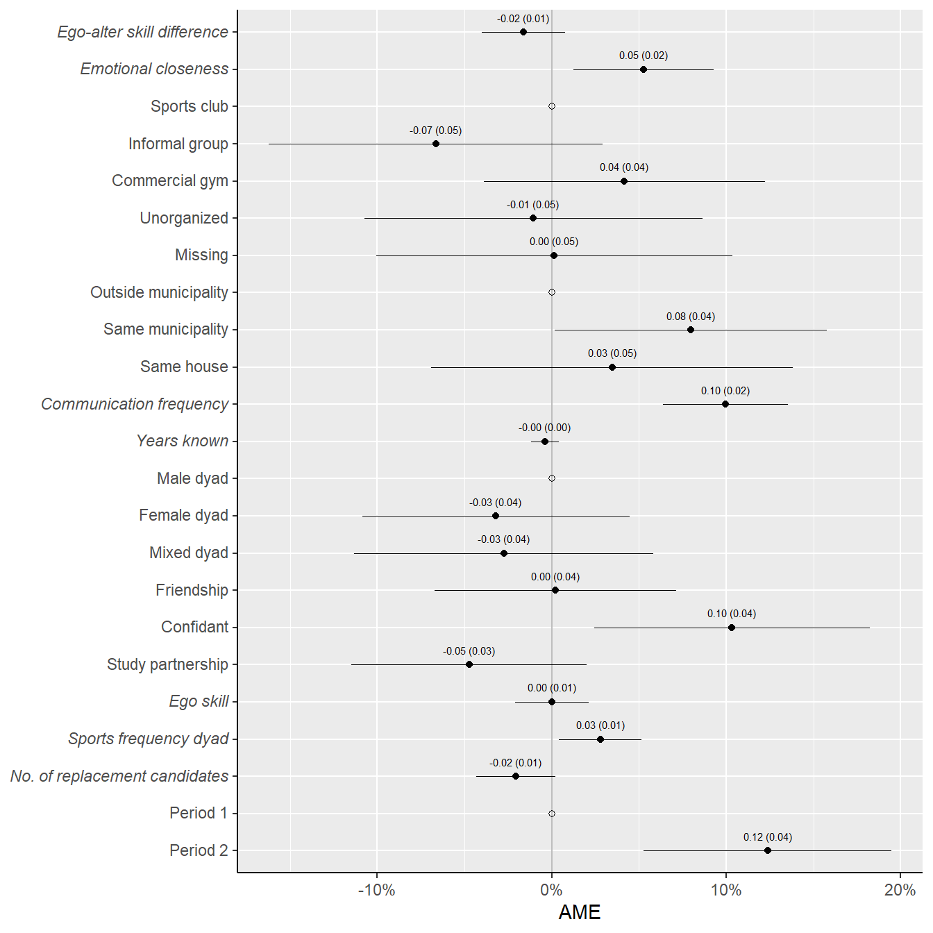
LS0tDQp0aXRsZTogIkFuYWx5c2lzIg0KYmlibGlvZ3JhcGh5OiByZWZlcmVuY2VzLmJpYg0KbGluay1jaXRhdGlvbnM6IHRydWUNCmRhdGU6ICJMYXN0IGNvbXBpbGVkIG9uIGByIGZvcm1hdChTeXMudGltZSgpLCAnJUIsICVZJylgIg0Kb3V0cHV0OiANCiAgaHRtbF9kb2N1bWVudDoNCiAgICBjc3M6IHR3ZWFrcy5jc3MNCiAgICB0b2M6ICB0cnVlDQogICAgdG9jX2Zsb2F0OiB0cnVlDQogICAgbnVtYmVyX3NlY3Rpb25zOiB0cnVlDQogICAgdG9jX2RlcHRoOiAyDQogICAgY29kZV9mb2xkaW5nOiBzaG93DQogICAgY29kZV9kb3dubG9hZDogeWVzDQotLS0NCg0KYGBge3IsIGdsb2JhbHNldHRpbmdzLCBlY2hvPUZBTFNFLCB3YXJuaW5nPUZBTFNFLCByZXN1bHRzPSdoaWRlJyxtZXNzYWdlPUZBTFNFfQ0KbGlicmFyeShrbml0cikNCmxpYnJhcnkodGlkeXZlcnNlKQ0Ka25pdHI6Om9wdHNfY2h1bmskc2V0KGVjaG8gPSBUUlVFKQ0Kb3B0c19jaHVuayRzZXQodGlkeS5vcHRzPWxpc3Qod2lkdGguY3V0b2ZmPTEwMCksdGlkeT1UUlVFLCB3YXJuaW5nID0gRkFMU0UsIG1lc3NhZ2UgPSBGQUxTRSxjb21tZW50ID0gIiM+IiwgY2FjaGU9VFJVRSwgY2xhc3Muc291cmNlPWMoInRlc3QiKSwgY2xhc3Mub3V0cHV0PWMoInRlc3QzIikpDQpvcHRpb25zKHdpZHRoID0gMTAwKQ0KcmdsOjpzZXR1cEtuaXRyKCkNCg0KY29sb3JpemUgPC0gZnVuY3Rpb24oeCwgY29sb3IpIHtzcHJpbnRmKCI8c3BhbiBzdHlsZT0nY29sb3I6ICVzOyc+JXM8L3NwYW4+IiwgY29sb3IsIHgpIH0NCmBgYA0KDQoNCmBgYHtyIGtsaXBweSwgZWNobz1GQUxTRSwgaW5jbHVkZT1UUlVFfQ0Ka2xpcHB5OjprbGlwcHkocG9zaXRpb24gPSBjKCd0b3AnLCAncmlnaHQnKSkNCiNrbGlwcHk6OmtsaXBweShjb2xvciA9ICdkYXJrcmVkJykNCiNrbGlwcHk6OmtsaXBweSh0b29sdGlwX21lc3NhZ2UgPSAnQ2xpY2sgdG8gY29weScsIHRvb2x0aXBfc3VjY2VzcyA9ICdEb25lJykNCmBgYA0KDQoNCg0KLS0tICANCiAgDQojIEdldHRpbmcgc3RhcnRlZA0KDQpUbyBjb3B5IHRoZSBjb2RlLCBjbGljayB0aGUgYnV0dG9uIGluIHRoZSB1cHBlciByaWdodCBjb3JuZXIgb2YgdGhlIGNvZGUtY2h1bmtzLg0KDQojIyBjbGVhbiB1cA0KDQpgYGB7ciwgZXZhbD1GQUxTRSwgcmVzdWx0cz0naGlkZSd9DQpybShsaXN0PWxzKCkpDQpnYygpDQpgYGANCg0KPGJyPg0KDQojIyBnZW5lcmFsIGN1c3RvbSBmdW5jdGlvbnMNCg0KLSBgZnBhY2thZ2UuY2hlY2tgOiBDaGVjayBpZiBwYWNrYWdlcyBhcmUgaW5zdGFsbGVkIChhbmQgaW5zdGFsbCBpZiBub3QpIGluIFINCi0gYGZzYXZlYDogRnVuY3Rpb24gdG8gc2F2ZSBkYXRhIHdpdGggdGltZSBzdGFtcCBpbiBjb3JyZWN0IGRpcmVjdG9yeQ0KLSBgZmxvYWRgOiBGdW5jdGlvbiB0byBsb2FkIFItb2JqZWN0cyB1bmRlciBuZXcgbmFtZXMNCi0gYGZ0aGVtZWA6IHByZXR0eSBnZ3Bsb3QyIHRoZW1lDQotIGBmc2hvd2RmYDogUHJpbnQgb2JqZWN0cyAoYHRpYmJsZWAgLyBgZGF0YS5mcmFtZWApIG5pY2VseSBvbiBzY3JlZW4gaW4gYC5SbWRgLg0KLSBgZmZpdGA6IGZpdCBhIHNlcmllcyBvZiAoaGVyZSwgZ2VuZXJhbGl6ZWQgbGluZWFyIG1peGVkLWVmZmVjdHMpIG1vZGVscyANCg0KYGBge3J9DQpmcGFja2FnZS5jaGVjayA8LSBmdW5jdGlvbihwYWNrYWdlcykgew0KICAgIGxhcHBseShwYWNrYWdlcywgRlVOID0gZnVuY3Rpb24oeCkgew0KICAgICAgICBpZiAoIXJlcXVpcmUoeCwgY2hhcmFjdGVyLm9ubHkgPSBUUlVFKSkgew0KICAgICAgICAgICAgaW5zdGFsbC5wYWNrYWdlcyh4LCBkZXBlbmRlbmNpZXMgPSBUUlVFKQ0KICAgICAgICAgICAgbGlicmFyeSh4LCBjaGFyYWN0ZXIub25seSA9IFRSVUUpDQogICAgICAgIH0NCiAgICB9KQ0KfQ0KDQpmc2F2ZSA8LSBmdW5jdGlvbih4LCBmaWxlLCBsb2NhdGlvbiA9ICIuL2RhdGEvcHJvY2Vzc2VkLyIsIC4uLikgew0KICAgIGlmICghZGlyLmV4aXN0cyhsb2NhdGlvbikpDQogICAgICAgIGRpci5jcmVhdGUobG9jYXRpb24pDQogICAgZGF0ZW5hbWUgPC0gc3Vic3RyKGdzdWIoIls6LV0iLCAiIiwgU3lzLnRpbWUoKSksIDEsIDgpDQogICAgdG90YWxuYW1lIDwtIHBhc3RlKGxvY2F0aW9uLCBkYXRlbmFtZSwgZmlsZSwgc2VwID0gIiIpDQogICAgcHJpbnQocGFzdGUoIlNBVkVEOiAiLCB0b3RhbG5hbWUsIHNlcCA9ICIiKSkNCiAgICBzYXZlKHgsIGZpbGUgPSB0b3RhbG5hbWUpDQp9DQoNCmZsb2FkICA8LSBmdW5jdGlvbihmaWxlTmFtZSl7DQogIGxvYWQoZmlsZU5hbWUpDQogIGdldChscygpW2xzKCkgIT0gImZpbGVOYW1lIl0pDQp9DQoNCiNleHRyYWZvbnQ6OmZvbnRfaW1wb3J0KHBhdGhzID0gYygiQzovVXNlcnMvdTI0NDE0Ny9Eb3dubG9hZHMvSm9zdC8iLCBwcm9tcHQgPSBGQUxTRSkpDQpmdGhlbWUgPC0gZnVuY3Rpb24oKSB7DQogIA0KICAjZG93bmxvYWQgZm9udCBhdCBodHRwczovL2ZvbnRzLmdvb2dsZS5jb20vc3BlY2ltZW4vSm9zdC8NCiAgdGhlbWVfbWluaW1hbChiYXNlX2ZhbWlseSA9ICJKb3N0IikgKw0KICAgIHRoZW1lKHBhbmVsLmdyaWQubWlub3IgPSBlbGVtZW50X2JsYW5rKCksDQogICAgICAgICAgcGxvdC50aXRsZSA9IGVsZW1lbnRfdGV4dChmYW1pbHkgPSAiSm9zdCIsIGZhY2UgPSAiYm9sZCIpLA0KICAgICAgICAgIGF4aXMudGl0bGUgPSBlbGVtZW50X3RleHQoZmFtaWx5ID0gIkpvc3QgTWVkaXVtIiksDQogICAgICAgICAgYXhpcy50aXRsZS54ID0gZWxlbWVudF90ZXh0KGhqdXN0ID0gMCksDQogICAgICAgICAgYXhpcy50aXRsZS55ID0gZWxlbWVudF90ZXh0KGhqdXN0ID0gMSksDQogICAgICAgICAgc3RyaXAudGV4dCA9IGVsZW1lbnRfdGV4dChmYW1pbHkgPSAiSm9zdCIsIGZhY2UgPSAiYm9sZCIsDQogICAgICAgICAgICAgICAgICAgICAgICAgICAgICAgICAgICBzaXplID0gcmVsKDAuNzUpLCBoanVzdCA9IDApLA0KICAgICAgICAgIHN0cmlwLmJhY2tncm91bmQgPSBlbGVtZW50X3JlY3QoZmlsbCA9ICJncmV5OTAiLCBjb2xvciA9IE5BKSwNCiAgICAgICAgICBsZWdlbmQucG9zaXRpb24gPSAiYm90dG9tIikNCn0NCg0KZnNob3dkZiA8LSBmdW5jdGlvbih4LCBkaWdpdHMgPSAyLCAuLi4pIHsNCiAgICBrbml0cjo6a2FibGUoeCwgZGlnaXRzID0gZGlnaXRzLCAiaHRtbCIsIC4uLikgJT4lDQogICAgICAgIGthYmxlRXh0cmE6OmthYmxlX3N0eWxpbmcoYm9vdHN0cmFwX29wdGlvbnMgPSBjKCJzdHJpcGVkIiwgImhvdmVyIikpICU+JQ0KICAgICAgICBrYWJsZUV4dHJhOjpzY3JvbGxfYm94KHdpZHRoID0gIjEwMCUiLCBoZWlnaHQgPSAiMzAwcHgiKQ0KfQ0KDQpmZml0IDwtIGZ1bmN0aW9uKGZvcm11bGEsIGRhdGEpIHsNCiAgdHJ5Q2F0Y2goew0KICAgIG1vZGVsIDwtIGxtZTQ6OmdsbWVyKGZvcm11bGEsIGRhdGEgPSBkYXRhLCBmYW1pbHkgPSBiaW5vbWlhbChsaW5rID0gImxvZ2l0IiksDQogICAgICAgICAgICAgICAgICAgY29udHJvbCA9IGdsbWVyQ29udHJvbChvcHRpbWl6ZXIgPSAiYm9ieXFhIiwgb3B0Q3RybCA9IGxpc3QobWF4ZnVuID0gMWU1KSkpDQogICAgY2F0KCJGaXR0aW5nIG1vZGVsOiIsIGFzLmNoYXJhY3Rlcihmb3JtdWxhKSwgIlxuIikNCiAgICBzdW1tYXJ5KG1vZGVsKQ0KICAgIGNhdCgiXG4iKQ0KICAgIHJldHVybihtb2RlbCkNCiAgfSwgZXJyb3IgPSBmdW5jdGlvbihlKSB7DQogICAgY2F0KCJFcnJvciBmaXR0aW5nIG1vZGVsOiIsIGFzLmNoYXJhY3Rlcihmb3JtdWxhKSwgIlxuIikNCiAgICBjYXQoIkVycm9yIG1lc3NhZ2U6IiwgY29uZGl0aW9uTWVzc2FnZShlKSwgIlxuIikNCiAgICByZXR1cm4oTlVMTCkNCiAgfSkNCn0NCmBgYA0KDQpgYGB7ciBmb250cywgZWNobz1GQUxTRSwgd2FybmluZz1GQUxTRSwgcmVzdWx0cz0naGlkZSd9DQojIGltcG9ydCBmb250IEpPU1QNCiNleHRyYWZvbnQ6OmZvbnRfaW1wb3J0KHBhdHRlcm4gPSAiSm9zdCIpDQpleHRyYWZvbnQ6OmxvYWRmb250cyhkZXZpY2U9IndpbiIpDQoNCiMgU2V0IGRlZmF1bHQgdGhlbWUgYW5kIGZvbnQgc3R1ZmYNCnRoZW1lX3NldChmdGhlbWUoKSkNCnVwZGF0ZV9nZW9tX2RlZmF1bHRzKCJ0ZXh0IiwgbGlzdChmYW1pbHkgPSAiSm9zdCIsIGZvbnRmYWNlID0gInBsYWluIikpDQp1cGRhdGVfZ2VvbV9kZWZhdWx0cygibGFiZWwiLCBsaXN0KGZhbWlseSA9ICJKb3N0IiwgZm9udGZhY2UgPSAicGxhaW4iKSkNCg0KI25pY2UgY29sb3IgcGFsZXR0ZQ0KY2JQYWxldHRlIDwtIGMoIiM5OTk5OTkiLCAiI0U2OUYwMCIsICIjNTZCNEU5IiwgIiMwMDlFNzMiLCAiI0YwRTQ0MiIsICIjMDA3MkIyIiwgIiNENTVFMDAiLCAiI0NDNzlBNyIpDQpgYGANCg0KPGJyPg0KDQoNCiMjIG5lY2Vzc2FyeSBwYWNrYWdlcw0KDQotIGB0aWR5dmVyc2VgDQotIGBsbWU0YDogZml0dGluZyByYW5kb20gZWZmZWN0cyBtb2RlbHMNCi0gYGxtdGVzdGA6IGRpYWdub3N0aWNzIHRlc3QgKGxpa2VsaWhvb2QgcmF0aW8gdGVzdCkNCi0gYGNhcmA6IGNvbXBhbmlvbiBhcHBsaWVkIHJlZ3Jlc3Npb24gKGNhbGN1bGF0ZSBWSUYpDQotIGB0ZXhyZWdgOiBvdXRwdXQgdG8gSFRNTCB0YWJsZQ0KLSBgZ2dwbG90MmAgDQotIGBnZ3B1YnJgOiBmb3JtYXQgZ2dwbG90MiBwbG90cw0KLSBgZ2doNHhgOiBoYWNrcyBmb3IgZ2dwbG90Mg0KLSBgZ2d0ZXh0YDogdGV4dCByZW5kZXJpbmcNCi0gYHBhcmFsbGVsYDogcGFyYWxsZWwgY29tcHV0aW5nDQoNCg0KYGBge3IsIHJlc3VsdHM9J2hpZGUnLCBtZXNzYWdlPUZBTFNFLCB3YXJuaW5nPUZBTFNFfQ0KcGFja2FnZXMgPSBjKCJ0aWR5dmVyc2UiLCAibG1lNCIsImxtdGVzdCIsImNhciIsInRleHJlZyIsImdncGxvdDIiLCJnZ3B1YnIiLCJnZ2g0eCIsImdndGV4dCIsICJwYXJhbGxlbCIpDQpmcGFja2FnZS5jaGVjayhwYWNrYWdlcykNCnJtKHBhY2thZ2VzKQ0KYGBgIA0KDQo8YnI+DQoNCiMjIGxvYWQgZGF0YS1zZXQNCg0KTG9hZCB0aGUgcmVwbGljYXRlZCBkYXRhLXNldC4gVG8gbG9hZCB0aGVzZSBmaWxlLCBhZGp1c3QgdGhlIGZpbGVuYW1lIGluIHRoZSBmb2xsb3dpbmcgY29kZSBzbyB0aGF0IGl0IG1hdGNoZXMgdGhlIG1vc3QgcmVjZW50IHZlcnNpb24gb2YgdGhlIGAuUkRhYCBmaWxlIHlvdSBoYXZlIGluIHlvdXIgYC4vZGF0YS9wcm9jZXNzZWQvYCBmb2xkZXIuDQoNCllvdSBtYXkgYWxzbyBvYnRhaW4gdGhlbSBieSBkb3dubG9hZGluZzogYHIgeGZ1bjo6ZW1iZWRfZmlsZSgiLi9kYXRhIHNoYXJlZC9uZXR3b3JrZGF0YS5SZGEiKWANCg0KDQpgYGB7ciwgcmVzdWx0cyA9ICdoaWRlJ30NCiNsaXN0IGZpbGVzIGluIHByb2Nlc3NlZCBkYXRhIGZvbGRlcg0KbGlzdC5maWxlcygiLi9kYXRhL3Byb2Nlc3NlZC8iKQ0KDQojZ2V0IHRvZGF5cyBkYXRlOg0KdG9kYXkgPC0gZ3N1YigiLSIsICIiLCBTeXMuRGF0ZSgpKQ0KDQojdXNlIGZsb2FkDQpkZiA8LSBmbG9hZChwYXN0ZTAoIi4vZGF0YS9wcm9jZXNzZWQvIiwgdG9kYXksICJuZXR3b3JrZGF0YS5SZGEiKSkNCmBgYA0KDQoNCg0KPGJyPg0KDQojIyBsYXN0IGFsdGVyYXRpb25zDQoNCi0gc3Vic2V0IHNwb3J0cyBwYXJ0bmVycyBhdCB0IHRvIHN0dWR5IHRpZSBtYWludGVuYW5jZSBhdCB0KzENCi0gYmluYXJ5IG91dGNvbWUgKHNwb3J0cyBwYXJ0bmVyOiB5ZXMvbm87IDEvMCkNCi0gY2FsY3VsYXRlIG5vLiBvZiAncmVwbGFjZW1lbnQgY2FuZGlkYXRlcycgKGkuZS4sIG5vLiBvZiBvdGhlciBzcG9ydHMgcGFydG5lcnMsIG90aGVyIHRoYW4gYWx0ZXIgaiwgd2l0aCB3aG9tIGVnbyBkb2VzIHRoZSBzcG9ydCB0eXBlIGhlL3NoZSBkb2VzIHdpdGggYWx0ZXIpDQotIHByb3hpbWl0eSBsZXZlbHMNCi0gc3BvcnRzIHNldHRpbmdzDQotIGR5YWRpYyBza2lsbCBjYXRlZ29yeSBjb21iaW5hdGlvbnMgKEhILCBITSwgSEwsIE1MLCBNTSwgTEwpDQotIGFsc28gZGlmZmVyZW5jZSBzY29yZSBpbiBza2lsbA0KLSBhbHRlciBzcG9ydHMgZnJlcXVlbmN5IGFuZCBlZ28vYWx0ZXIgbWVhbg0KLSBnZW5kZXIgY29tcG9zaXRpb24gZHlhZCAoTU0sIEZNLCBGRikNCi0gdHlwZSBvZiBzcG9ydCAoZml0bmVzcywgZW5kdXJhbmNlLCB0ZWFtLCBtaXNjZWxsYW5lb3VzKQ0KDQpgYGB7cn0NCiNzdWJzZXQgc3BvcnRzIHBhcnRuZXJzIGF0IHQNCmRmIDwtIGRmW2RmJGNzbiA9PSAxLF0NCg0KI291dGNvbWUNCmRmJHkgPC0gaWZlbHNlKGRmJFljc24gPT0gMSwgMSwgMCkNCg0KI2NhbGN1bGF0ZSBycGVsYWNlbWVudCBjYW5kaWRhdGVzOiBuby4gb2Ygb3RoZXIgc3BvcnRzIHBhcnRuZXJzIG5leHQgdG8gYWx0ZXIgaiwgYXQgdGltZSB0LCB3aXRoIHdob20gZWdvIGRvZXMgdGhlIHNhbWUgYWN0aXZpdHkgdHlwZQ0KZGYkbnJlcGxhY2UgPC0gTkENCg0KZm9yIChpIGluIHVuaXF1ZShkZiRlZ28pKSB7IA0KICBmb3IgKHQgaW4gdW5pcXVlKGRmJHBlcmlvZFtkZiRlZ28gPT0gaV0pKSB7IA0KICAgIGZvciAoaiBpbiB1bmlxdWUoZGYkYWx0ZXJpZFtkZiRlZ28gPT0gaSAmIGRmJHBlcmlvZCA9PSB0XSkpIHsNCiAgICANCiAgICAgICNnZXQgYWN0aXZpdHkgdHlwZSBhbHRlciBqIGRvZXMgd2l0aCBlZ28gYXQgdA0KICAgICAgYWN0aXZpdHkgPC0gZGYkc3BvcnR0b2dldGhlcltkZiRlZ28gPT0gaSAmIGRmJGFsdGVyaWQgPT0gaiAmIGRmJHBlcmlvZCA9PSB0XQ0KICAgIA0KICAgICAgI2dldCBudW1iZXIgb2YgKm90aGVyKiBhbHRlcnMgd2l0aCB3aG9tIGVnbyBkb2VzIHRoZSBzYW1lIGFjdGl2aXR5IGF0IHQgKGllLCByZXBsYWNlbWVudCBjYW5kaWRhdGVzKQ0KICAgICAgZGYkbnJlcGxhY2VbZGYkZWdvID09IGkgJiBkZiRhbHRlcmlkID09IGogJiBkZiRwZXJpb2QgPT0gdF0gPC0gbGVuZ3RoKHdoaWNoKGRmJHNwb3J0dG9nZXRoZXJbZGYkZWdvID09IGkgJiAhZGYkYWx0ZXJpZCA9PSBqICYgZGYkcGVyaW9kID09IHRdID09IGFjdGl2aXR5KSkNCiAgICB9DQogIH0NCn0NCg0KZGYkcHJveGltaXR5IDwtIGZhY3RvcihkZiRwcm94aW1pdHksIGxldmVscyA9IGMoImZhciIsImNsb3NlIiwicm9vbW1hdGUiKSkNCmRmJGNsb3NlIDwtIGlmZWxzZShkZiRwcm94aW1pdHkgPT0gImNsb3NlIiwxLDApDQpkZiRyb29tbWF0ZSA8LSBpZmVsc2UoZGYkcHJveGltaXR5ID09ICJyb29tbWF0ZSIsMSwwKQ0KZGYkZmFyIDwtIGlmZWxzZShkZiRwcm94aW1pdHkgPT0gImZhciIsMSwwKQ0KDQpkZiRlZ29fY29udGV4dFtpcy5uYShkZiRlZ29fY29udGV4dCldIDwtICJtaXNzaW5nIg0KZGYkZWdvX2NvbnRleHQgPC0gZmFjdG9yKGRmJGVnb19jb250ZXh0LCBsZXZlbHMgPSBjKCJjbHViIiwgImluZm9ybWFsIiwgImd5bSIsICJhbG9uZSIsICJtaXNzaW5nIikpDQpkZiRjbHViIDwtIGlmZWxzZShkZiRlZ29fY29udGV4dCA9PSAiY2x1YiIsMSwwKQ0KZGYkaW5mb3JtYWwgPC0gaWZlbHNlKGRmJGVnb19jb250ZXh0ID09ICJpbmZvcm1hbCIsMSwwKQ0KZGYkZ3ltIDwtIGlmZWxzZShkZiRlZ29fY29udGV4dCA9PSAiZ3ltIiwxLDApDQpkZiRhbG9uZSA8LSBpZmVsc2UoZGYkZWdvX2NvbnRleHQgPT0gImFsb25lIiwxLDApDQpkZiRtaXNzaW5nIDwtIGlmZWxzZShkZiRlZ29fY29udGV4dCA9PSAibWlzc2luZyIsMSwwKQ0KDQpkZiRISCA8LSBpZmVsc2UoZGYkZWdvX2dyYWRlID4gNyAmIGRmJGFsdGVyX2dyYWRlID4gNywgMSwgMCkNCmRmJEhNIDwtIGlmZWxzZSggKChkZiRlZ29fZ3JhZGUgPiA3ICYgZGYkYWx0ZXJfZ3JhZGUgPiA1ICYgZGYkYWx0ZXJfZ3JhZGUgPCA4KSB8IChkZiRhbHRlcl9ncmFkZSA+IDcgJiBkZiRlZ29fZ3JhZGUgPiA1ICYgZGYkZWdvX2dyYWRlIDwgOCkpLCAxLCAwKQ0KZGYkSEwgPC0gaWZlbHNlKCAoKGRmJGVnb19ncmFkZSA+IDcgJiBkZiRhbHRlcl9ncmFkZSA8IDYpIHwgKGRmJGFsdGVyX2dyYWRlID4gNyAmIGRmJGVnb19ncmFkZSA8IDYpKSwgMSwgMCkNCmRmJE1NIDwtIGlmZWxzZSggKChkZiRlZ29fZ3JhZGUgPiA1ICYgZGYkZWdvX2dyYWRlIDwgOCAmIGRmJGFsdGVyX2dyYWRlID4gNSAmIGRmJGFsdGVyX2dyYWRlIDwgOCkpLCAxLCAwKQ0KZGYkTUwgPC0gaWZlbHNlKCAoKGRmJGVnb19ncmFkZSA+IDUgJiBkZiRlZ29fZ3JhZGUgPCA4ICYgZGYkYWx0ZXJfZ3JhZGUgPCA2KSB8IChkZiRlZ29fZ3JhZGUgPCA2ICYgZGYkYWx0ZXJfZ3JhZGUgPCA4ICYgZGYkYWx0ZXJfZ3JhZGUgPiA1KSksIDEsIDApDQpkZiRMTCA8LSBpZmVsc2UoICgoZGYkZWdvX2dyYWRlIDwgNiAmIGRmJGFsdGVyX2dyYWRlIDwgNikpLCAxLCAwKQ0KDQpkZiRza2lsbHMgPC0gZmFjdG9yKA0KICAxICogKCgoZGYkZWdvX2dyYWRlID4gNSAmIGRmJGVnb19ncmFkZSA8IDggJiBkZiRhbHRlcl9ncmFkZSA+IDUgJiBkZiRhbHRlcl9ncmFkZSA8IDgpKSkgKyAgIyBNTQ0KICAyICogKGRmJGVnb19ncmFkZSA+IDcgJiBkZiRhbHRlcl9ncmFkZSA+IDcpICsgICAgICAgICMgSEgNCiAgMyAqICgoKGRmJGVnb19ncmFkZSA+IDcgJiBkZiRhbHRlcl9ncmFkZSA+IDUgJiBkZiRhbHRlcl9ncmFkZSA8IDgpIHwgKGRmJGFsdGVyX2dyYWRlID4gNyAmIGRmJGVnb19ncmFkZSA+IDUgJiBkZiRlZ29fZ3JhZGUgPCA4KSkpICsgICMgSE0NCiAgNCAqICgoKGRmJGVnb19ncmFkZSA+IDcgJiBkZiRhbHRlcl9ncmFkZSA8IDYpIHwgKGRmJGFsdGVyX2dyYWRlID4gNyAmIGRmJGVnb19ncmFkZSA8IDYpKSkgKyAgIyBITA0KICA1ICogKCgoZGYkZWdvX2dyYWRlID4gNSAmIGRmJGVnb19ncmFkZSA8IDggJiBkZiRhbHRlcl9ncmFkZSA8IDYpIHwgKGRmJGVnb19ncmFkZSA8IDYgJiBkZiRhbHRlcl9ncmFkZSA8IDggJiBkZiRhbHRlcl9ncmFkZSA+IDUpKSkgKyAgIyBNTA0KICA2ICogKCgoZGYkZWdvX2dyYWRlIDwgNiAmIGRmJGFsdGVyX2dyYWRlIDwgNikpKSwgICAgICAgICMgTEwNCiAgbGV2ZWxzID0gYygxLCAyLCAzLCA0LCA1LCA2KSwNCiAgbGFiZWxzID0gYygiTU0iLCAiSEgiLCAiSE0iLCAiSEwiLCAiTUwiLCAiTEwiKQ0KKQ0KDQpkZiRkaWZfc2tpbGwgPC0gYWJzKGRmJGVnb19ncmFkZSAtIGRmJGFsdGVyX2dyYWRlKQ0KDQpkZiRhbHRlcl9mcmVxMiA8LSBpZmVsc2UoZGYkYWx0ZXJfZnJlcSA9PSAiMSBrZWVyIHBlciB3ZWVrIiwgMSwNCiAgICAgICAgICAgICAgICAgICAgICAgIGlmZWxzZShkZiRhbHRlcl9mcmVxID09ICIyIG9mIDMga2VlciBwZXIgd2VlayIsIDIuNSwNCiAgICAgICAgICAgICAgICAgICAgICAgICAgICAgaWZlbHNlKGRmJGFsdGVyX2ZyZXEgPT0gIjQgb2YgNSBrZWVyIHBlciB3ZWVrIiwgNC41LA0KICAgICAgICAgICAgICAgICAgICAgICAgICAgICAgICAgICAgaWZlbHNlKGRmJGFsdGVyX2ZyZXEgPT0gIjYga2VlciBwZXIgd2VlayBvZiB2YWtlciIsIDYuNSwNCiAgICAgICAgICAgICAgICAgICAgICAgICAgICAgICAgICAgICAgICAgICBpZmVsc2UoZGYkYWx0ZXJfZnJlcSA9PSAiTWluZGVyIGRhbiAxIGtlZXIgcGVyIG1hYW5kIiwgMC4xMjUsDQogICAgICAgICAgICAgICAgICAgICAgICAgICAgICAgICAgICAgICAgICAgICAgICAgIGlmZWxzZShkZiRhbHRlcl9mcmVxID09ICIxIG9mIDIga2VlciBwZXIgbWFhbmQiLCAwLjM3NSwNCiAgICAgICAgICAgICAgICAgICAgICAgICAgICAgICAgICAgICAgICAgICAgICAgICAgICAgICAgIGlmZWxzZShkZiRhbHRlcl9mcmVxID09ICIxIG9mIDIga2VlciBwZXIgbWFhbmQiLCAwLjM3NSwgTkEpKSkpKSkpDQpkZiRlZ29fZnJlcSA8LSBhcy5udW1lcmljKGRmJGVnb19mcmVxKQ0KZGYkZWdvX2FjdGl2ZXcxIDwtIGlmZWxzZShkZiRlZ29fbWVhbmZyZXEgPjAsIDEsIDApDQoNCmRmIDwtIGRmICU+JQ0KICBtdXRhdGUobWVhbl9mcmVxID0gcm93TWVhbnMoc2VsZWN0KC4sIGFsdGVyX2ZyZXEyLCBlZ29fZnJlcSksIG5hLnJtID0gVFJVRSkpDQoNCiNkZiRlZ29fbWVhbnNraWxsW2lzLm5hKGRmJGVnb19tZWFuc2tpbGwpXSA8LSBtZWFuKGRmJGVnb19tZWFuc2tpbGxbd2hpY2goIWR1cGxpY2F0ZWQoZGYkZWdvKSldLCBuYS5ybT1UUlVFICkNCg0KZGYkYWx0ZXJfYWdlIDwtIGFzLm51bWVyaWMoZGYkYWx0ZXJfYWdlKQ0KDQpkZiRmZiA8LSBpZmVsc2UoZGYkZWdvX2ZlbWFsZSA9PSAxICYgZGYkYWx0ZXJfZmVtYWxlID09IDEsIDEsIDApDQpkZiRmbSA8LSBpZmVsc2UoICgoZGYkZWdvX2ZlbWFsZSA9PSAxICYgZGYkYWx0ZXJfZmVtYWxlID09IDApIHwgKGRmJGVnb19mZW1hbGUgPT0gMCAmIGRmJGFsdGVyX2ZlbWFsZSA9PSAxKSksIDEsIDApDQpkZiRtbSA8LSBpZmVsc2UoZGYkZWdvX2ZlbWFsZSA9PSAwICYgZGYkYWx0ZXJfZmVtYWxlID09IDAsIDEsIDApDQoNCmRmJGdlbmRlciA8LSBmYWN0b3IoDQogIDEgKiAoZGYkZWdvX2ZlbWFsZSA9PSAwICYgZGYkYWx0ZXJfZmVtYWxlID09IDApICsgICMgTU0NCiAgMiAqICgoZGYkZWdvX2ZlbWFsZSA9PSAxICYgZGYkYWx0ZXJfZmVtYWxlID09IDApIHwgKGRmJGVnb19mZW1hbGUgPT0gMCAmIGRmJGFsdGVyX2ZlbWFsZSA9PSAxKSkgKyAgIyBGTQ0KICAzICogKGRmJGVnb19mZW1hbGUgPT0gMSAmIGRmJGFsdGVyX2ZlbWFsZSA9PSAxKSwgICMgRkYNCiAgbGV2ZWxzID0gYygxLCAyLCAzKSwNCiAgbGFiZWxzID0gYygiTU0iLCAiRk0iLCAiRkYiKQ0KKQ0KDQpkZiRlZ29fcXVpdFtpcy5uYShkZiRlZ29fcXVpdCldIDwtIDANCg0KI2V4Y2x1ZGUga2luDQpkZltkZiRraW4gPT0gIjAiLF0gLT4gZGYNCg0KI3R5cGVzIG9mIHNwb3J0DQpkZiRmaXRuZXNzIDwtIGlmZWxzZShkZiRzcG9ydHRvZ2V0aGVyID09IDEsMSwwKQ0KZGYkZW5kdXJhbmNlIDwtIGlmZWxzZShkZiRzcG9ydHRvZ2V0aGVyICVpbiUgYygyLDUsNyksIDEsIDApDQpkZiR0ZWFtIDwtIGlmZWxzZShkZiRzcG9ydHRvZ2V0aGVyICVpbiUgYygzLDEwLDEyKSwgMSwgMCkNCmRmJG1pc2MgPC0gaWZlbHNlKCFkZiRzcG9ydHRvZ2V0aGVyICVpbiUgYygxLDIsNSw3LDMsMTAsMTIpLDEsMCkNCg0KZGYkc3BvcnR0eXBlIDwtIGZhY3RvcigNCiAgMSAqIChkZiRmaXRuZXNzID09IDEpICsNCiAgMiAqIChkZiRlbmR1cmFuY2UgPT0gMSkgKw0KICAzICogKGRmJHRlYW0gPT0gMSkgKw0KICA0ICogKGRmJG1pc2MgPT0gMSksDQogIGxldmVscyA9IGMoMTo0KSwNCiAgbGFiZWxzID0gYygiZml0bmVzcyIsICJlbmR1cmFuY2UiLCAidGVhbSIsICJtaXNjZWxsYW5lb3VzIikNCikNCmBgYA0KDQotLS0NCg0KPGJyPg0KDQojIERlc2NyaXB0aXZlcw0KDQpgYGB7ciwgZXZhbD1UUlVFfQ0KI2xpc3R3aXNlIGRlbGV0aW9uDQpkZiAlPiUgDQogIHNlbGVjdChwcm94aW1pdHksIHJvb21tYXRlLCBjbG9zZSwgZmFyLCBmcmVxdWVuY3kudCwgY2xvc2VuZXNzLnQsIGR1cmF0aW9uLCBjc24sIGJmZiwgc3R1ZHksIGNkbiwgZ2VuZGVyLCBtbSwgZm0sIGZmLCBwZXJpb2QsIHksIGVnbywgYWx0ZXJpZCwgZWdvX2FjdGl2ZXcxLA0KICAgICAgICAgbWVhbl9mcmVxLCBza2lsbHMsIEhILCBITSwgSEwsIE1NLCBNTCwgTEwsIGVnb19ncmFkZSwgZGlmX3NraWxsLCBlZ29fY29udGV4dCwgY2x1YiwgaW5mb3JtYWwsIGd5bSwgYWxvbmUsIG1pc3NpbmcsIHNwb3J0dG9nZXRoZXIsIG5yZXBsYWNlLCBzcG9ydHR5cGUsIGZpdG5lc3MsIGVuZHVyYW5jZSwgdGVhbSwgbWlzYykgJT4lDQogIGZpbHRlcihjb21wbGV0ZS5jYXNlcyguKSkgLT4gZGYNCg0KI2Rlc2NyaWJlDQpkZiAlPiUNCiAgc2VsZWN0KC1jKHByb3hpbWl0eSwgZ2VuZGVyLCBza2lsbHMsIGVnb19jb250ZXh0LCBlZ28sIGFsdGVyaWQsIGVnb19hY3RpdmV3MSwgc3BvcnR0b2dldGhlciwgc3BvcnR0eXBlKSkgJT4lDQogIHBzeWNoOjpkZXNjcmliZSgpICU+JQ0KICBmc2hvd2RmKGNhcHRpb249ImRlc2NyaXB0aXZlIHN0YXRpc3RpY3Mgb2YgZWdvJ3MgKG5vbi1raW4pIHNvY2lhbCByZWxhdGlvbnMgV0lUSElOIFNQT1JUUyBhdCB0aW1lIHQiKQ0KDQpsZW5ndGgodW5pcXVlKHBhc3RlMChkZiRlZ28sIlgiLGRmJGFsdGVyaWQpKSkgI05fYWx0ZXIgPTEyMjINCm5yb3coZGYpICNOX29ic2VydmF0aW9uID0gMTQyNg0KYGBgDQoNCjxicj4NCg0KLS0tLQ0KDQojIE11bHRpdmFyaWF0ZSBhbmFseXNlcw0KDQojIyBsb2dpc3RpYyByZWdyZXNzaW9uDQoNCmBgYHtyLGV2YWw9RkFMU0V9DQojdGllIGNvbnRpbnVhdGlvbjoNCg0KZm9ybXVsYSA8LSBsaXN0KA0KICAjbW9kZWwgMTogbWFpbiBwcmVkaWN0b3JzDQogIHkgfiAxICsgKDEgfCBlZ28pICsgc2NhbGUoZWdvX2dyYWRlKSArIHNjYWxlKGRpZl9za2lsbCkgKyBzY2FsZShjbG9zZW5lc3MudCkgKyBlZ29fY29udGV4dCArIGFzLmZhY3RvcihwZXJpb2QpLA0KICANCiAgI21vZGVsIDI6IGNvbnRyb2wgZm9yIHNwb3J0cyBiZWhhdmlvciBkeWFkDQogIHkgfiAxICsgKDEgfCBlZ28pICsgc2NhbGUoZWdvX2dyYWRlKSArIHNjYWxlKGRpZl9za2lsbCkgKyBzY2FsZShjbG9zZW5lc3MudCkgKyBlZ29fY29udGV4dCArIGFzLmZhY3RvcihwZXJpb2QpICsgc2NhbGUobWVhbl9mcmVxKSwNCiAgDQogICNtb2RlbCAzOiBpbmNsdWRlICJ0cmFkaXRpb25hbCIgZHlhZGljIGNvbnRyb2xzDQogIHkgfiAxICsgKDEgfCBlZ28pICsgc2NhbGUoZWdvX2dyYWRlKSArIHNjYWxlKGRpZl9za2lsbCkgKyBzY2FsZShjbG9zZW5lc3MudCkgKyBlZ29fY29udGV4dCArIGFzLmZhY3RvcihwZXJpb2QpICsgc2NhbGUobWVhbl9mcmVxKSArIHByb3hpbWl0eSArIHNjYWxlKGZyZXF1ZW5jeS50KSArIHNjYWxlKGR1cmF0aW9uKSArIGdlbmRlciwNCiAgDQogICNtb2RlbCA0OiBhZGQgb3RoZXIgcmVsYXRpb25hbCBkaW1lbnNpb25zIChtdWx0aXBsZXhpdHkpDQogIHkgfiAxICsgKDEgfCBlZ28pICsgc2NhbGUoZWdvX2dyYWRlKSArIHNjYWxlKGRpZl9za2lsbCkgICsgc2NhbGUoY2xvc2VuZXNzLnQpICsgZWdvX2NvbnRleHQgKyBhcy5mYWN0b3IocGVyaW9kKSArIHNjYWxlKG1lYW5fZnJlcSkgKyBwcm94aW1pdHkgKyBzY2FsZShmcmVxdWVuY3kudCkgKyBzY2FsZShkdXJhdGlvbikgKyBnZW5kZXIgKyBiZmYgKyBjZG4gKyBzdHVkeSwNCiAgDQogICNtb2RlbCA1OiBhZGQgcmVwbGFjZW1lbnQgY2FuZGlkYXRlcw0KICB5IH4gMSArICgxIHwgZWdvKSArIHNjYWxlKGVnb19ncmFkZSkgKyBzY2FsZShkaWZfc2tpbGwpICsgc2NhbGUoY2xvc2VuZXNzLnQpICsgZWdvX2NvbnRleHQgKyBhcy5mYWN0b3IocGVyaW9kKSArIHNjYWxlKG1lYW5fZnJlcSkgKyBwcm94aW1pdHkgKyBzY2FsZShmcmVxdWVuY3kudCkgKyBzY2FsZShkdXJhdGlvbikgKyBnZW5kZXIgKyBiZmYgKyBjZG4gKyBzdHVkeSArIHNjYWxlKG5yZXBsYWNlKQ0KICApDQoNCmFucyA8LSBsYXBwbHkoZm9ybXVsYSwgZmZpdCwgZGF0YSA9IGRmKQ0KbGFwcGx5KGFucywgc3VtbWFyeSkNCmRvLmNhbGwobG10ZXN0OjpscnRlc3QsYW5zKQ0KYGBgDQoNCmBgYHtyLCBldmFsPUZBTFNFLCBlY2hvPUZBTFNFfQ0KdGV4cmVnOjpodG1scmVnKGFucywNCiAgICAgICAgZmlsZT0iLi9yZXN1bHRzL2NvZWZ0YWJfbWFpbnRlbmFuY2UuaHRtbCIsDQogICAgICAgIGNhcHRpb249IlJlc3VsdHMgb2YgcmFuZG9tIGVmZmVjdHMgbW9kZWxzIHByZWRpY3Rpbmcgc3BvcnRzIHBhcnRuZXJzaGlwIG1haW50ZW5hbmNlIGF0IHQrMSAoMT15ZXMsIDA9bm8pIiwgY2FwdGlvbi5hYm92ZSA9IFRSVUUsDQogICAgICAgIGN1c3RvbS5tb2RlbC5uYW1lcyA9IGMoIk0xOiBtYWluIHByZWRpY3RvcnMiLCAiTTI6IHNwb3J0cyBiZWguIGR5YWQiLCAiTTM6IGR5YWRpYyBjb3ZhcnMiLCAiTTQ6IG11bHRpcGxleGl0eSIsICJNNTogcmVwbGFjZW1lbnQgY2FuZGlkYXRlcyIpLA0KICAgICAgIGN1c3RvbS5jb2VmLm5hbWVzID0gYygiKEludGVyY2VwdCkiLCANCiAgICAgICAgICAgICAgICAgICAgICAgICAgICAgIkVnbyBza2lsbCIsICJFZ28tYWx0ZXIgc2tpbGwgZGlmZXJlbmNlIiwgDQogICAgICAgICAgICAgICAgICAgICAgICAgICAgICJFbW90aW9uYWwgY2xvc2VuZXNzIiwgIkluZm9ybWFsIGdyb3VwIiwgIkNvbW1lcmNpYWwgZ3ltIiwgIlVub3JnYW5pemVkIiwgIk1pc3NpbmciLCANCiAgICAgICAgICAgICAgICAgICAgICAgICAgICAgIlBlcmlvZDogd2F2ZXMgMi0zIiwgICJNZWFuIHNwb3J0cyBmcmVxdWVuY3kgZHlhZCIsICJTYW1lIG11bmljaXBhbGl0eSIsICJSb29tbWF0ZSIsICJDb21tdW5pY2F0aW9uIGZyZXF1ZW5jeSIsICJZZWFycyBrbm93biIsDQogICAgICAgICAgICAgICAgICAgICAgICAgICAgICJXb21hbi1tYW4iLCAiV29tYW4td29tYW4iLCAiRnJpZW5kc2hpcCIsICJDb25maWRhbnQiLCAiU3R1ZHkgcGFydG5lciIsICJOby4gb2YgcmVwbGFjZW1lbnQgY2FuZGlkYXRlcyIpLA0KICAgICAgIGRpZ2l0cz0yLCBzaW5nbGUucm93ID0gVFJVRQ0KICAgICAgICApDQpgYGANCg0KPGJyPg0KDQojIyBvdXRwdXQNCg0KYGBge3IsIGVjaG8gPSBGQUxTRX0NCmh0bWx0b29sczo6dGFncyRkaXYoDQogIHN0eWxlID0gImhlaWdodDogNjAwcHg7IG92ZXJmbG93LXk6IHNjcm9sbDsiLA0KICBodG1sdG9vbHM6OmluY2x1ZGVIVE1MKCIuL3Jlc3VsdHMvY29lZnRhYl9tYWludGVuYW5jZS5odG1sIikNCikNCmBgYA0KDQo8YnI+DQoNCiMjIHJvYnVzdG5lc3MgY2hlY2tzDQoNCiMjIyBwYXR0ZXJucyBkZXBlbmQgb24gdHlwZSBvZiBzcG9ydD8gey50YWJzZXQgLnRhYnNldC1mYWRlfQ0KDQpXZSBjb21wYXJlIHJlc3VsdHMgaW4gc3BvcnRzIHBhcnRuZXJzaGlwcyBpbiB2cy4gb3V0c2lkZSBmaXRuZXNzLg0KDQpgYGB7ciwgZXZhbD1GQUxTRX0NCmRmICU+JQ0KICBzZWxlY3Qoc3BvcnR0b2dldGhlcikgJT4lDQogIHRhYmxlKC4pICU+JQ0KICBwcm9wLnRhYmxlKC4pDQoNCiNvZiBhbGwgc3BvcnRzIHBhcnRuZXIgb2JzZXJ2YXRpb25zOg0KIzI3JSBhcmUgaW4gZml0bmVzczsgdGhpcyBpcyB0aGUgbW9zdCBwb3B1bGFyIHNwb3J0cyBpbiBkeWFkcw0KIzExJSBhcmUgaW4gZW5kdXJhbmNlIHNwb3J0cyAoaS5lLiwgcnVubmluZywgY3ljbGluZywgc3dpbW1pbmcpDQojMTUlIGFyZSBpbiB0ZWFtIChiYWxsKSBzcG9ydHMgKGkuZS4sIGZvb3RiYWxsLCBob2NrZXksIHZvbGxleWJhbCkNCg0KIzEuIHNvbHV0aW9uIGZvciBmaXRuZXNzIHBhcnRuZXJzOg0KYW5zX2ZpdG5lc3MgPC0gbGFwcGx5KGZvcm11bGEsIGZmaXQsIGRhdGEgPSBkZltkZiRzcG9ydHRvZ2V0aGVyID09IDEsXSkNCmxhcHBseShhbnNfZml0bmVzcywgc3VtbWFyeSkNCg0KIzIuIHNvbHV0aW9uIGV4Y2x1ZGluZyBmaXRuZXNzIHBhcnRuZXJzOg0KYW5zX25maXRuZXNzIDwtIGxhcHBseShmb3JtdWxhLCBmZml0LCBkYXRhID0gZGZbIWRmJHNwb3J0dG9nZXRoZXIgPT0gMSxdKQ0KbGFwcGx5KGFuc19uZml0bmVzcywgc3VtbWFyeSkNCg0KIzMuIHNvbHV0aW9uIGZvciBlbmR1cmFuY2Ugc3BvcnRzIHBhcnRuZXJzOg0KYW5zX2VuZHVyYW5jZSA8LSBsYXBwbHkoZm9ybXVsYSwgZmZpdCwgZGF0YSA9IGRmW2RmJHNwb3J0dG9nZXRoZXIgJWluJSBjKDIsNSw3KSxdKQ0KbGFwcGx5KGFuc19lbmR1cmFuY2UsIHN1bW1hcnkpDQoNCiM0LiBzb2x1dGlvbiBmb3IgdGVhbSAoYmFsbCkgc3BvcnRzIHBhcnRuZXJzOg0KYW5zX3RlYW0gPC0gbGFwcGx5KGZvcm11bGEsIGZmaXQsIGRhdGEgPSBkZltkZiRzcG9ydHRvZ2V0aGVyICVpbiUgYygzLDEwLDEyKSxdKQ0KbGFwcGx5KGFuc190ZWFtLCBzdW1tYXJ5KQ0KYGBgDQoNCmBgYHtyLCBldmFsPUZBTFNFLCBlY2hvPUZBTFNFfQ0KdGV4cmVnOjpodG1scmVnKGFuc19maXRuZXNzLA0KICAgICAgICBmaWxlPSIuL3Jlc3VsdHMvY29lZnRhYl9maXRuZXNzLmh0bWwiLA0KICAgICAgICBjYXB0aW9uPSJSZXN1bHRzIG9mIHJhbmRvbSBlZmZlY3RzIG1vZGVscyBwcmVkaWN0aW5nIHNwb3J0cyBwYXJ0bmVyc2hpcCBtYWludGVuYW5jZSBJTiBGSVRORVNTIGF0IHQrMSAoMT15ZXMsIDA9bm8pIiwgY2FwdGlvbi5hYm92ZSA9IFRSVUUsDQogICAgICAgIGN1c3RvbS5tb2RlbC5uYW1lcyA9IGMoIk0xOiBtYWluIHByZWRpY3RvcnMiLCAiTTI6IHNwb3J0cyBiZWguIGR5YWQiLCAiTTM6IGR5YWRpYyBjb3ZhcnMiLCAiTTQ6IG11bHRpcGxleGl0eSIsICJNNTogcmVwbGFjZW1lbnQgY2FuZGlkYXRlcyIpLA0KICAgICAgIGN1c3RvbS5jb2VmLm5hbWVzID0gYygiKEludGVyY2VwdCkiLCANCiAgICAgICAgICAgICAgICAgICAgICAgICAgICAgIkVnbyBza2lsbCIsICJFZ28tYWx0ZXIgc2tpbGwgZGlmZXJlbmNlIiwgDQogICAgICAgICAgICAgICAgICAgICAgICAgICAgICJFbW90aW9uYWwgY2xvc2VuZXNzIiwgIkluZm9ybWFsIGdyb3VwIiwgIkNvbW1lcmNpYWwgZ3ltIiwgIlVub3JnYW5pemVkIiwgIk1pc3NpbmciLCANCiAgICAgICAgICAgICAgICAgICAgICAgICAgICAgIlBlcmlvZDogd2F2ZXMgMi0zIiwgICJNZWFuIHNwb3J0cyBmcmVxdWVuY3kgZHlhZCIsICJTYW1lIG11bmljaXBhbGl0eSIsICJSb29tbWF0ZSIsICJDb21tdW5pY2F0aW9uIGZyZXF1ZW5jeSIsICJZZWFycyBrbm93biIsDQogICAgICAgICAgICAgICAgICAgICAgICAgICAgICJXb21hbi1tYW4iLCAiV29tYW4td29tYW4iLCAiRnJpZW5kc2hpcCIsICJDb25maWRhbnQiLCAiU3R1ZHkgcGFydG5lciIsICJOby4gb2YgcmVwbGFjZW1lbnQgY2FuZGlkYXRlcyIpLA0KICAgICAgIGRpZ2l0cz0yLCBzaW5nbGUucm93ID0gVFJVRQ0KICAgICAgICApDQoNCnRleHJlZzo6aHRtbHJlZyhhbnNfbmZpdG5lc3MsDQogICAgICAgIGZpbGU9Ii4vcmVzdWx0cy9jb2VmdGFiX25maXRuZXNzLmh0bWwiLA0KICAgICAgICBjYXB0aW9uPSJSZXN1bHRzIG9mIHJhbmRvbSBlZmZlY3RzIG1vZGVscyBwcmVkaWN0aW5nIHNwb3J0cyBwYXJ0bmVyc2hpcCBtYWludGVuYW5jZSBPVVRTSURFIEZJVE5FU1MgYXQgdCsxICgxPXllcywgMD1ubykiLCBjYXB0aW9uLmFib3ZlID0gVFJVRSwNCiAgICAgICAgY3VzdG9tLm1vZGVsLm5hbWVzID0gYygiTTE6IG1haW4gcHJlZGljdG9ycyIsICJNMjogc3BvcnRzIGJlaC4gZHlhZCIsICJNMzogZHlhZGljIGNvdmFycyIsICJNNDogbXVsdGlwbGV4aXR5IiwgIk01OiByZXBsYWNlbWVudCBjYW5kaWRhdGVzIiksDQogICAgICAgICAgICAgIGN1c3RvbS5jb2VmLm5hbWVzID0gYygiKEludGVyY2VwdCkiLCANCiAgICAgICAgICAgICAgICAgICAgICAgICAgICAgIkVnbyBza2lsbCIsICJFZ28tYWx0ZXIgc2tpbGwgZGlmZXJlbmNlIiwgDQogICAgICAgICAgICAgICAgICAgICAgICAgICAgICJFbW90aW9uYWwgY2xvc2VuZXNzIiwgIkluZm9ybWFsIGdyb3VwIiwgIkNvbW1lcmNpYWwgZ3ltIiwgIlVub3JnYW5pemVkIiwgIk1pc3NpbmciLA0KICAgICAgICAgICAgICAgICAgICAgICAgICAgICAiUGVyaW9kOiB3YXZlcyAyLTMiLCAgIk1lYW4gc3BvcnRzIGZyZXF1ZW5jeSBkeWFkIiwgIlNhbWUgbXVuaWNpcGFsaXR5IiwgIlJvb21tYXRlIiwgIkNvbW11bmljYXRpb24gZnJlcXVlbmN5IiwgIlllYXJzIGtub3duIiwNCiAgICAgICAgICAgICAgICAgICAgICAgICAgICAgIldvbWFuLW1hbiIsICJXb21hbi13b21hbiIsICJGcmllbmRzaGlwIiwgIkNvbmZpZGFudCIsICJTdHVkeSBwYXJ0bmVyIiwgIk5vLiBvZiByZXBsYWNlbWVudCBjYW5kaWRhdGVzIiksDQogICAgICAgZGlnaXRzPTIsIHNpbmdsZS5yb3cgPSBUUlVFDQogICAgICAgICkNCmBgYA0KDQo8YnI+DQoNCiMjIyMgc3BvcnRzIHBhcnRuZXJzIGluIGZpdG5lc3MNCg0KYGBge3IsIGVjaG8gPSBGQUxTRX0NCmh0bWx0b29sczo6dGFncyRkaXYoDQogIHN0eWxlID0gImhlaWdodDogNjAwcHg7IG92ZXJmbG93LXk6IHNjcm9sbDsiLA0KICBodG1sdG9vbHM6OmluY2x1ZGVIVE1MKCIuL3Jlc3VsdHMvY29lZnRhYl9maXRuZXNzLmh0bWwiKQ0KKQ0KYGBgDQoNCjxicj4NCg0KIyMjIyBzcG9ydHMgcGFydG5lcnMgb3V0c2lkZSBmaXRuZXNzDQoNCmBgYHtyLCBlY2hvID0gRkFMU0V9DQpodG1sdG9vbHM6OnRhZ3MkZGl2KA0KICBzdHlsZSA9ICJoZWlnaHQ6IDYwMHB4OyBvdmVyZmxvdy15OiBzY3JvbGw7IiwNCiAgaHRtbHRvb2xzOjppbmNsdWRlSFRNTCgiLi9yZXN1bHRzL2NvZWZ0YWJfbmZpdG5lc3MuaHRtbCIpDQopDQpgYGANCg0KPCEtLS0gDQoNCg0KIyMjIHsudW5saXN0ZWQgLnVubnVtYmVyZWR9DQoNCjxicj4NCg0KIyMjIHNraWxsIGxldmVsIGRpZmZlcmVuY2Ugc2NvcmUNCg0KV2UgdXNlIGFuIGFsdGVybmF0aXZlIG1lYXN1cmUgb2YgZHlhZGljIHNraWxsIGxldmVsIGRpZmZlcmVuY2VzOiBXZSBpbmNsdWRlIHRoZSBhYnNvbHV0ZSBkaWZmZXJlbmNlIGJldHdlZW4gZWdvIGFuZCBhbHRlciwgYW5kIHdlIGNvbnRyb2wgZm9yIGVnbydzIHNraWxsIGxldmVsLg0KDQpgYGB7ciwgZXZhbD1GQUxTRX0NCmZvcm11bGEyIDwtIGxpc3QoDQogICNtb2RlbCAxOiBtYWluIHByZWRpY3RvcnMNCiAgeSB+IDEgKyAoMSB8IGVnbykgKyBzY2FsZShlZ29fZ3JhZGUpICsgc2NhbGUoZGlmX3NraWxsKSArIHNjYWxlKGNsb3NlbmVzcy50KSArIGVnb19jb250ZXh0ICsgYXMuZmFjdG9yKHBlcmlvZCksDQogIA0KICAjbW9kZWwgMjogY29udHJvbCBmb3Igc3BvcnRzIGJlaGF2aW9yIGR5YWQNCiAgeSB+IDEgKyAoMSB8IGVnbykgKyAgc2NhbGUoZWdvX2dyYWRlKSAgKyBzY2FsZShkaWZfc2tpbGwpICArIHNjYWxlKGNsb3NlbmVzcy50KSArIGVnb19jb250ZXh0ICsgYXMuZmFjdG9yKHBlcmlvZCkgKyBlZ29fcXVpdCArIHNjYWxlKG1lYW5fZnJlcSksDQogIA0KICAjbW9kZWwgMzogaW5jbHVkZSAidHJhZGl0aW9uYWwiIGR5YWRpYyBjb250cm9scw0KICB5IH4gMSArICgxIHwgZWdvKSArICBzY2FsZShlZ29fZ3JhZGUpICArIHNjYWxlKGRpZl9za2lsbCkgICArIHNjYWxlKGNsb3NlbmVzcy50KSArIGVnb19jb250ZXh0ICsgYXMuZmFjdG9yKHBlcmlvZCkgKyBlZ29fcXVpdCArIHNjYWxlKG1lYW5fZnJlcSkgKyBwcm94aW1pdHkgKyBzY2FsZShmcmVxdWVuY3kudCkgKyBzY2FsZShkdXJhdGlvbikgKyBnZW5kZXIsDQogIA0KICAjbW9kZWwgNDogYWRkIG90aGVyIHJlbGF0aW9uYWwgZGltZW5zaW9ucyAobXVsdGlwbGV4aXR5KQ0KICB5IH4gMSArICgxIHwgZWdvKSArICBzY2FsZShlZ29fZ3JhZGUpICArIHNjYWxlKGRpZl9za2lsbCkgICArIHNjYWxlKGNsb3NlbmVzcy50KSArIGVnb19jb250ZXh0ICsgYXMuZmFjdG9yKHBlcmlvZCkgKyBlZ29fcXVpdCArIHNjYWxlKG1lYW5fZnJlcSkgKyBwcm94aW1pdHkgKyBzY2FsZShmcmVxdWVuY3kudCkgKyBzY2FsZShkdXJhdGlvbikgKyBnZW5kZXIgKyBiZmYgKyBjZG4gKyBzdHVkeSwNCiAgDQogICNtb2RlbCA1OiBhZGQgcmVwbGFjZW1lbnQgY2FuZGlkYXRlcw0KICB5IH4gMSArICgxIHwgZWdvKSArICBzY2FsZShlZ29fZ3JhZGUpICArIHNjYWxlKGRpZl9za2lsbCkgICArIHNjYWxlKGNsb3NlbmVzcy50KSArIGVnb19jb250ZXh0ICsgYXMuZmFjdG9yKHBlcmlvZCkgKyBlZ29fcXVpdCArIHNjYWxlKG1lYW5fZnJlcSkgKyBwcm94aW1pdHkgKyBzY2FsZShmcmVxdWVuY3kudCkgKyBzY2FsZShkdXJhdGlvbikgKyBnZW5kZXIgKyBiZmYgKyBjZG4gKyBzdHVkeSArIHNjYWxlKG5yZXBsYWNlKQ0KICApDQoNCiNlc3RpbWF0ZQ0KYW5zX3NraWxsZGlmIDwtIGxhcHBseShmb3JtdWxhMiwgZmZpdCwgZGF0YSA9IGRmKQ0KbGFwcGx5KGFuc19za2lsbGRpZiwgc3VtbWFyeSkNCmBgYA0KDQpgYGB7ciwgZXZhbD1GQUxTRSwgZWNobz1GQUxTRX0NCnRleHJlZzo6aHRtbHJlZyhhbnNfc2tpbGxkaWYsDQogICAgICAgIGZpbGU9Ii4vcmVzdWx0cy9jb2VmdGFiX3NraWxsZGlmLmh0bWwiLA0KICAgICAgICBjYXB0aW9uPSJSZXN1bHRzIG9mIHJhbmRvbSBlZmZlY3RzIG1vZGVscyBwcmVkaWN0aW5nIHNwb3J0cyBwYXJ0bmVyc2hpcCBtYWludGVuYW5jZSBhdCB0KzEgKDE9eWVzLCAwPW5vKTsgd2l0aCBhbHRlcm5hdGl2ZSBvcGVyYXRpb25hbGl6YXRpb24gZm9yIGR5YWRpYyBza2lsbHMgZ2FwIiwgY2FwdGlvbi5hYm92ZSA9IFRSVUUsDQogICAgICAgIGN1c3RvbS5tb2RlbC5uYW1lcyA9IGMoIk0xOiBtYWluIHByZWRpY3RvcnMiLCAiTTI6IHNwb3J0cyBiZWguIGR5YWQiLCAiTTM6IGR5YWRpYyBjb3ZhcnMiLCAiTTQ6IG11bHRpcGxleGl0eSIsICJNNTogcmVwbGFjZW1lbnQgY2FuZGlkYXRlcyIpLA0KICAgICAgIGN1c3RvbS5jb2VmLm5hbWVzID0gYygiKEludGVyY2VwdCkiLCANCiAgICAgICAgICAgICAgICAgICAgICAgICAgICAgIkVnbyBza2lsbHMiLCAiQWJzb2x1dGUgZHlhZGljIHNraWxsIGRpZmZlcmVuY2UiLCANCiAgICAgICAgICAgICAgICAgICAgICAgICAgICAgIkVtb3Rpb25hbCBjbG9zZW5lc3MiLCAiSW5mb3JtYWwgZ3JvdXAiLCAiQ29tbWVyY2lhbCBneW0iLCAiVW5vcmdhbml6ZWQiLCAiTWlzc2luZyIsIA0KICAgICAgICAgICAgICAgICAgICAgICAgICAgICAiUGVyaW9kOiB3YXZlcyAyLTMiLCAiRWdvIHF1aXQgYXQgdCsxIiwgIk1lYW4gc3BvcnRzIGZyZXF1ZW5jeSBkeWFkIiwgIlNhbWUgbXVuaWNpcGFsaXR5IiwgIlJvb21tYXRlIiwgIkNvbW11bmljYXRpb24gZnJlcXVlbmN5IiwgIlllYXJzIGtub3duIiwNCiAgICAgICAgICAgICAgICAgICAgICAgICAgICAgIldvbWFuLW1hbiIsICJXb21hbi13b21hbiIsICJGcmllbmRzaGlwIiwgIkNvbmZpZGFudCIsICJTdHVkeSBwYXJ0bmVyIiwgIk5vLiBvZiByZXBsYWNlbWVudCBjYW5kaWRhdGVzIiksDQogICAgICAgZGlnaXRzPTIsIHNpbmdsZS5yb3cgPSBUUlVFDQogICAgICAgICkNCmBgYA0KDQpgYGB7ciwgZWNobyA9IEZBTFNFfQ0KaHRtbHRvb2xzOjp0YWdzJGRpdigNCiAgc3R5bGUgPSAiaGVpZ2h0OiA2MDBweDsgb3ZlcmZsb3cteTogc2Nyb2xsOyIsDQogIGh0bWx0b29sczo6aW5jbHVkZUhUTUwoIi4vcmVzdWx0cy9jb2VmdGFiX3NraWxsZGlmLmh0bWwiKQ0KKQ0KYGBgDQoNCg0KLS0+DQoNCi0tLQ0KDQoNCjxicj4NCg0KIyMgQU1Fcw0KDQpGb3IgbW9yZSBpbmZvcm1hdGlvbiBvbiB0aGUgKG51bWVyaWNhbCkgYXBwcm9hY2ggdG8gY29tcHV0aW5nIEFNRXMsIHNlZSBodHRwczovL3d3dy5qb2NoZW10b2xzbWEubmwvdHV0b3JpYWxzL21lLy4NCg0KIyMjIyBkZWZpbmUgZGF0YS1zZXRzDQoNCmBgYHtyLCBldmFsPUZBTFNFfQ0KIzIuIHRpZSBtYWludGVuYW5jZQ0KZGZjbG9zZTEgPC0gZGZjbG9zZTAgPC0gZGYNCmRmcm9vbW1hdGUxIDwtIGRmcm9vbW1hdGUwIDwtIGRmDQoNCmRmY2xvc2UxJHByb3hpbWl0eSA8LSAiY2xvc2UiDQpkZmNsb3NlMCRwcm94aW1pdHkgPC0gImZhciINCmRmcm9vbW1hdGUxJHByb3hpbWl0eSA8LSAicm9vbW1hdGUiDQpkZnJvb21tYXRlMCRwcm94aW1pdHkgPC0gImZhciINCg0KcyA8LSAwLjAwMQ0KZGZjbG9zZW5lc3NwbHVzIDwtIGRmY2xvc2VuZXNzbWluIDwtIGRmDQpkZmNsb3NlbmVzc3BsdXMkY2xvc2VuZXNzLnQgPC0gZGYkY2xvc2VuZXNzLnQgKyBzDQpkZmNsb3NlbmVzc21pbiRjbG9zZW5lc3MudCA8LSBkZiRjbG9zZW5lc3MudCAtIHMNCg0KZGZmcmllbmQxIDwtIGRmZnJpZW5kMCA8LSBkZg0KZGZzdHVkeTEgPC0gZGZzdHVkeTAgPC0gZGYNCmRmY2RuMSA8LSBkZmNkbjAgPC0gZGYNCmRmZnJpZW5kMSRiZmYgPC0gMQ0KZGZmcmllbmQwJGJmZiA8LSAwDQpkZnN0dWR5MSRzdHVkeSA8LSAxDQpkZnN0dWR5MCRzdHVkeSA8LSAwDQpkZmNkbjEkY2RuIDwtIDENCmRmY2RuMCRjZG4gPC0gMA0KDQpkZndvbWVuMSA8LSBkZndvbWVuMCA8LSBkZm1peGVkMSA8LSBkZm1peGVkMCA8LSBkZg0KZGZ3b21lbjEkZ2VuZGVyIDwtICJGRiINCmRmd29tZW4wJGdlbmRlciA8LSAiTU0iDQpkZm1peGVkMSRnZW5kZXIgPC0gIkZNIg0KZGZtaXhlZDAkZ2VuZGVyIDwtICJNTSINCg0KZGZkdXJhdGlvbnBsdXMgPC0gZGZkdXJhdGlvbm1pbiA8LSBkZg0KZGZkdXJhdGlvbnBsdXMkZHVyYXRpb24gPC0gZGYkZHVyYXRpb24gKyBzDQpkZmR1cmF0aW9ubWluJGR1cmF0aW9uIDwtIGRmJGR1cmF0aW9uIC0gcw0KDQpkZmZyZXF1ZW5jeXBsdXMgPC0gZGZmcmVxdWVuY3ltaW4gPC0gZGYNCmRmZnJlcXVlbmN5cGx1cyRmcmVxdWVuY3kudCA8LSBkZiRmcmVxdWVuY3kudCArIHMNCmRmZnJlcXVlbmN5bWluJGZyZXF1ZW5jeS50IDwtIGRmJGZyZXF1ZW5jeS50IC0gcw0KDQpkZnBlcmlvZDIxIDwtIGRmcGVyaW9kMjAgPC0gZGYNCmRmcGVyaW9kMjEkcGVyaW9kIDwtIDINCmRmcGVyaW9kMjAkcGVyaW9kIDwtIDENCg0KZGZtZWFuZnJlcXBsdXMgPC0gZGZtZWFuZnJlcW1pbiA8LSBkZg0KZGZtZWFuZnJlcXBsdXMkbWVhbl9mcmVxIDwtIGRmJG1lYW5fZnJlcSArIHMNCmRmbWVhbmZyZXFtaW4kbWVhbl9mcmVxIDwtIGRmJG1lYW5fZnJlcSAtIHMNCg0KI2RmcXVpdDEgPC0gZGZxdWl0MCA8LSBkZg0KI2RmcXVpdDEkZWdvX3F1aXQgPC0gMQ0KI2RmcXVpdDAkZWdvX3F1aXQgPC0gMA0KDQojZGZISDEgPC0gZGZISDAgPC0gZGZITTEgPC0gZGZITTAgPC0gZGZITDEgPC0gZGZITDAgPC0gZGZNTDEgPC0gZGZNTDAgPC0gZGZMTDEgPC0gZGZMTDAgPC0gZGYNCiNkZkhIMSRza2lsbHMgPC0gIkhIIg0KI2RmSEgwJHNraWxscyA8LSAiTU0iDQojZGZITTEkc2tpbGxzIDwtICJITSINCiNkZkhNMCRza2lsbHMgPC0gIk1NIg0KI2RmSEwxJHNraWxscyA8LSAiSEwiDQojZGZITDAkc2tpbGxzIDwtICJNTSINCiNkZk1MMSRza2lsbHMgPC0gIk1MIg0KI2RmTUwwJHNraWxscyA8LSAiTU0iDQojZGZMTDEkc2tpbGxzIDwtICJMTCINCiNkZkxMMCRza2lsbHMgPC0gIk1NIg0KDQpkZmVnb3NraWxscGx1cyA8LSBkZmVnb3NraWxsbWluIDwtIGRmDQpkZmVnb3NraWxscGx1cyRlZ29fZ3JhZGUgPC0gZGYkZWdvX2dyYWRlICsgcw0KZGZlZ29za2lsbG1pbiRlZ29fZ3JhZGUgPC0gZGYkZWdvX2dyYWRlIC0gcw0KDQpkZnNraWxsZGlmcGx1cyA8LSBkZnNraWxsZGlmbWluIDwtIGRmDQpkZnNraWxsZGlmcGx1cyRkaWZfc2tpbGwgIDwtIGRmJGRpZl9za2lsbCArIHMNCmRmc2tpbGxkaWZtaW4kZGlmX3NraWxsICA8LSBkZiRkaWZfc2tpbGwgLSBzDQoNCmRmaW5mb3JtYWwxIDwtIGRmaW5mb3JtYWwwIDwtIGRmZ3ltMSA8LSBkZmd5bTAgPC0gZGZhbG9uZTEgPC0gZGZhbG9uZTAgPC0gZGZtaXNzaW5nMSA8LSBkZm1pc3NpbmcwIDwtIGRmDQpkZmluZm9ybWFsMSRlZ29fY29udGV4dCA8LSAiaW5mb3JtYWwiDQpkZmluZm9ybWFsMCRlZ29fY29udGV4dCA8LSAiY2x1YiINCmRmZ3ltMSRlZ29fY29udGV4dCA8LSAiZ3ltIg0KZGZneW0wJGVnb19jb250ZXh0IDwtICJjbHViIg0KZGZhbG9uZTEkZWdvX2NvbnRleHQgPC0gImFsb25lIg0KZGZhbG9uZTAkZWdvX2NvbnRleHQgPC0gImNsdWIiDQpkZm1pc3NpbmcxJGVnb19jb250ZXh0IDwtICJtaXNzaW5nIg0KZGZtaXNzaW5nMCRlZ29fY29udGV4dCA8LSAiY2x1YiINCg0KZGZyZXBsYWNlcGx1cyA8LSBkZnJlcGxhY2VtaW4gPC0gZGYNCmRmcmVwbGFjZXBsdXMkbnJlcGxhY2UgPC0gZGYkbnJlcGxhY2UgKyBzDQpkZnJlcGxhY2VtaW4kbnJlcGxhY2UgPC0gZGYkbnJlcGxhY2UgLSBzDQpgYGANCg0KPGJyPg0KDQojIyMjIGZ1bmN0aW9uIHRvIGNhbGN1bGF0ZSBBTUVzDQoNCmBgYHtyLCBldmFsPUZBTFNFfQ0KZnByZWQgPC0gZnVuY3Rpb24oeCkgew0KICBtZV9jbG9zZSA8LSBsbWU0Ojo6cHJlZGljdC5tZXJNb2QoeCwgdHlwZSA9ICJyZXNwb25zZSIsIHJlLmZvcm0gPSBOVUxMLCBuZXdkYXRhID0gZGZjbG9zZTEpIC0gbG1lNDo6OnByZWRpY3QubWVyTW9kKHgsIHR5cGUgPSAicmVzcG9uc2UiLCByZS5mb3JtID0gTlVMTCwgbmV3ZGF0YSA9IGRmY2xvc2UwKQ0KICBhbWVfY2xvc2UgPC0gbWVhbihtZV9jbG9zZSkNCiAgDQogIG1lX3Jvb21tYXRlIDwtIGxtZTQ6OjpwcmVkaWN0Lm1lck1vZCh4LCB0eXBlID0gInJlc3BvbnNlIiwgcmUuZm9ybSA9IE5VTEwsIG5ld2RhdGEgPSBkZnJvb21tYXRlMSkgLSBsbWU0Ojo6cHJlZGljdC5tZXJNb2QoeCwgdHlwZSA9ICJyZXNwb25zZSIsIHJlLmZvcm0gPSBOVUxMLCBuZXdkYXRhID0gZGZyb29tbWF0ZTApDQogIGFtZV9yb29tbWF0ZSA8LSBtZWFuKG1lX3Jvb21tYXRlKQ0KICANCiAgbWVfY2xvc2VuZXNzIDwtIChsbWU0Ojo6cHJlZGljdC5tZXJNb2QoeCwgdHlwZSA9ICJyZXNwb25zZSIsIHJlLmZvcm0gPSBOVUxMLCBuZXdkYXRhID0gZGZjbG9zZW5lc3NwbHVzKSAtIGxtZTQ6OjpwcmVkaWN0Lm1lck1vZCh4LCB0eXBlID0gInJlc3BvbnNlIiwgcmUuZm9ybSA9IE5VTEwsIG5ld2RhdGEgPSBkZmNsb3NlbmVzc21pbikpLygyICogcykNCiAgYW1lX2Nsb3NlbmVzcyA8LSBtZWFuKG1lX2Nsb3NlbmVzcykNCiAgDQogIG1lX2ZyaWVuZCA8LSBsbWU0Ojo6cHJlZGljdC5tZXJNb2QoeCwgdHlwZSA9ICJyZXNwb25zZSIsIHJlLmZvcm0gPSBOVUxMLCBuZXdkYXRhID0gZGZmcmllbmQxKSAtIGxtZTQ6OjpwcmVkaWN0Lm1lck1vZCh4LCB0eXBlID0gInJlc3BvbnNlIiwgcmUuZm9ybSA9IE5VTEwsIG5ld2RhdGEgPSBkZmZyaWVuZDApDQogIGFtZV9mcmllbmQgPC0gbWVhbihtZV9mcmllbmQpDQogIA0KICBtZV9zdHVkeSA8LSBsbWU0Ojo6cHJlZGljdC5tZXJNb2QoeCwgdHlwZSA9ICJyZXNwb25zZSIsIHJlLmZvcm0gPSBOVUxMLCBuZXdkYXRhID0gZGZzdHVkeTEpIC0gbG1lNDo6OnByZWRpY3QubWVyTW9kKHgsIHR5cGUgPSAicmVzcG9uc2UiLCByZS5mb3JtID0gTlVMTCwgbmV3ZGF0YSA9IGRmc3R1ZHkwKQ0KICBhbWVfc3R1ZHkgPC0gbWVhbihtZV9zdHVkeSkNCiAgDQogIG1lX2NkbiA8LSBsbWU0Ojo6cHJlZGljdC5tZXJNb2QoeCwgdHlwZSA9ICJyZXNwb25zZSIsIHJlLmZvcm0gPSBOVUxMLCBuZXdkYXRhID0gZGZjZG4xKSAtIGxtZTQ6OjpwcmVkaWN0Lm1lck1vZCh4LCB0eXBlID0gInJlc3BvbnNlIiwgcmUuZm9ybSA9IE5VTEwsIG5ld2RhdGEgPSBkZmNkbjApDQogIGFtZV9jZG4gPC0gbWVhbihtZV9jZG4pDQogIA0KICBtZV93b21lbiA8LSBsbWU0Ojo6cHJlZGljdC5tZXJNb2QoeCwgdHlwZSA9ICJyZXNwb25zZSIsIHJlLmZvcm0gPSBOVUxMLCBuZXdkYXRhID0gZGZ3b21lbjEpIC0gbG1lNDo6OnByZWRpY3QubWVyTW9kKHgsIHR5cGUgPSAicmVzcG9uc2UiLCByZS5mb3JtID0gTlVMTCwgbmV3ZGF0YSA9IGRmd29tZW4wKQ0KICBhbWVfd29tZW4gPC0gbWVhbihtZV93b21lbikNCiAgDQogIG1lX21peGVkIDwtIGxtZTQ6OjpwcmVkaWN0Lm1lck1vZCh4LCB0eXBlID0gInJlc3BvbnNlIiwgcmUuZm9ybSA9IE5VTEwsIG5ld2RhdGEgPSBkZm1peGVkMSkgLSBsbWU0Ojo6cHJlZGljdC5tZXJNb2QoeCwgdHlwZSA9ICJyZXNwb25zZSIsIHJlLmZvcm0gPSBOVUxMLCBuZXdkYXRhID0gZGZtaXhlZDApDQogIGFtZV9taXhlZCA8LSBtZWFuKG1lX21peGVkKQ0KICANCiAgbWVfZHVyYXRpb24gPC0gKGxtZTQ6OjpwcmVkaWN0Lm1lck1vZCh4LCB0eXBlID0gInJlc3BvbnNlIiwgcmUuZm9ybSA9IE5VTEwsIG5ld2RhdGEgPSBkZmR1cmF0aW9ucGx1cykgLSBsbWU0Ojo6cHJlZGljdC5tZXJNb2QoeCwgdHlwZSA9ICJyZXNwb25zZSIsIHJlLmZvcm0gPSBOVUxMLCBuZXdkYXRhID0gZGZkdXJhdGlvbm1pbikpLygyICogcykNCiAgYW1lX2R1cmF0aW9uIDwtIG1lYW4obWVfZHVyYXRpb24pDQogIA0KICBtZV9mcmVxdWVuY3kgPC0gKGxtZTQ6OjpwcmVkaWN0Lm1lck1vZCh4LCB0eXBlID0gInJlc3BvbnNlIiwgcmUuZm9ybSA9IE5VTEwsIG5ld2RhdGEgPSBkZmZyZXF1ZW5jeXBsdXMpIC0gbG1lNDo6OnByZWRpY3QubWVyTW9kKHgsIHR5cGUgPSAicmVzcG9uc2UiLCByZS5mb3JtID0gTlVMTCwgbmV3ZGF0YSA9IGRmZnJlcXVlbmN5bWluKSkvKDIgKiBzKQ0KICBhbWVfZnJlcXVlbmN5IDwtIG1lYW4obWVfZnJlcXVlbmN5KQ0KICANCiAgbWVfcGVyaW9kMiA8LSAgbG1lNDo6OnByZWRpY3QubWVyTW9kKHgsIHR5cGUgPSAicmVzcG9uc2UiLCByZS5mb3JtID0gTlVMTCwgbmV3ZGF0YSA9IGRmcGVyaW9kMjEpIC0gbG1lNDo6OnByZWRpY3QubWVyTW9kKHgsIHR5cGUgPSAicmVzcG9uc2UiLCByZS5mb3JtID0gTlVMTCwgbmV3ZGF0YSA9IGRmcGVyaW9kMjApDQogIGFtZV9wZXJpb2QyIDwtIG1lYW4obWVfcGVyaW9kMikNCiAgDQojICBtZV9xdWl0IDwtICBsbWU0Ojo6cHJlZGljdC5tZXJNb2QoeCwgdHlwZSA9ICJyZXNwb25zZSIsIHJlLmZvcm0gPSBOVUxMLCBuZXdkYXRhID0gZGZxdWl0MSkgLSBsbWU0Ojo6cHJlZGljdC5tZXJNb2QoeCwgI3R5cGUgPSAicmVzcG9uc2UiLCByZS5mb3JtID0gTlVMTCwgbmV3ZGF0YSA9IGRmcXVpdDApDQojICBhbWVfcXVpdCA8LSBtZWFuKG1lX3F1aXQpDQogIA0KIyAgbWVfSEggPC0gbG1lNDo6OnByZWRpY3QubWVyTW9kKHgsIHR5cGUgPSAicmVzcG9uc2UiLCByZS5mb3JtID0gTlVMTCwgbmV3ZGF0YSA9IGRmSEgxKSAtIGxtZTQ6OjpwcmVkaWN0Lm1lck1vZCh4LCB0eXBlID0gIyJyZXNwb25zZSIsIHJlLmZvcm0gPSBOVUxMLCBuZXdkYXRhID0gZGZISDApDQojICBhbWVfSEggPC0gbWVhbihtZV9ISCkNCiMgIG1lX0hNIDwtIGxtZTQ6OjpwcmVkaWN0Lm1lck1vZCh4LCB0eXBlID0gInJlc3BvbnNlIiwgcmUuZm9ybSA9IE5VTEwsIG5ld2RhdGEgPSBkZkhNMSkgLSBsbWU0Ojo6cHJlZGljdC5tZXJNb2QoeCwgdHlwZSA9ICMicmVzcG9uc2UiLCByZS5mb3JtID0gTlVMTCwgbmV3ZGF0YSA9IGRmSE0wKQ0KIyAgYW1lX0hNIDwtIG1lYW4obWVfSE0pDQojICBtZV9ITCA8LSBsbWU0Ojo6cHJlZGljdC5tZXJNb2QoeCwgdHlwZSA9ICJyZXNwb25zZSIsIHJlLmZvcm0gPSBOVUxMLCBuZXdkYXRhID0gZGZITDEpIC0gbG1lNDo6OnByZWRpY3QubWVyTW9kKHgsIHR5cGUgPSAjInJlc3BvbnNlIiwgcmUuZm9ybSA9IE5VTEwsIG5ld2RhdGEgPSBkZkhMMCkNCiMgIGFtZV9ITCA8LSBtZWFuKG1lX0hMKQ0KIyAgbWVfTUwgPC0gbG1lNDo6OnByZWRpY3QubWVyTW9kKHgsIHR5cGUgPSAicmVzcG9uc2UiLCByZS5mb3JtID0gTlVMTCwgbmV3ZGF0YSA9IGRmTUwxKSAtIGxtZTQ6OjpwcmVkaWN0Lm1lck1vZCh4LCB0eXBlID0gIyJyZXNwb25zZSIsIHJlLmZvcm0gPSBOVUxMLCBuZXdkYXRhID0gZGZNTDApDQojICBhbWVfTUwgPC0gbWVhbihtZV9NTCkNCiMgIG1lX0xMIDwtIGxtZTQ6OjpwcmVkaWN0Lm1lck1vZCh4LCB0eXBlID0gInJlc3BvbnNlIiwgcmUuZm9ybSA9IE5VTEwsIG5ld2RhdGEgPSBkZkxMMSkgLSBsbWU0Ojo6cHJlZGljdC5tZXJNb2QoeCwgdHlwZSA9ICMicmVzcG9uc2UiLCByZS5mb3JtID0gTlVMTCwgbmV3ZGF0YSA9IGRmTEwwKQ0KIyAgYW1lX0xMIDwtIG1lYW4obWVfTEwpDQogDQogIG1lX2Vnb3NraWxsIDwtIChsbWU0Ojo6cHJlZGljdC5tZXJNb2QoeCwgdHlwZSA9ICJyZXNwb25zZSIsIHJlLmZvcm0gPSBOVUxMLCBuZXdkYXRhID0gZGZlZ29za2lsbHBsdXMpIC0gbG1lNDo6OnByZWRpY3QubWVyTW9kKHgsIHR5cGUgPSAicmVzcG9uc2UiLCByZS5mb3JtID0gTlVMTCwgbmV3ZGF0YSA9IGRmZWdvc2tpbGxtaW4pKS8oMiAqIHMpDQogIGFtZV9lZ29za2lsbCA8LSBtZWFuKG1lX2Vnb3NraWxsKQ0KICANCiAgbWVfc2tpbGxkaWYgPC0gKGxtZTQ6OjpwcmVkaWN0Lm1lck1vZCh4LCB0eXBlID0gInJlc3BvbnNlIiwgcmUuZm9ybSA9IE5VTEwsIG5ld2RhdGEgPSBkZnNraWxsZGlmcGx1cykgLSBsbWU0Ojo6cHJlZGljdC5tZXJNb2QoeCwgdHlwZSA9ICJyZXNwb25zZSIsIHJlLmZvcm0gPSBOVUxMLCBuZXdkYXRhID0gZGZza2lsbGRpZm1pbikpLygyICogcykNCiAgYW1lX3NraWxsZGlmIDwtIG1lYW4obWVfc2tpbGxkaWYpDQogIA0KICAgDQogIG1lX2luZm9ybWFsIDwtIGxtZTQ6OjpwcmVkaWN0Lm1lck1vZCh4LCB0eXBlID0gInJlc3BvbnNlIiwgcmUuZm9ybSA9IE5VTEwsIG5ld2RhdGEgPSBkZmluZm9ybWFsMSkgLSBsbWU0Ojo6cHJlZGljdC5tZXJNb2QoeCwgdHlwZSA9ICJyZXNwb25zZSIsIHJlLmZvcm0gPSBOVUxMLCBuZXdkYXRhID0gZGZpbmZvcm1hbDApDQogIGFtZV9pbmZvcm1hbCA8LSBtZWFuKG1lX2luZm9ybWFsKQ0KICANCiAgbWVfZ3ltIDwtIGxtZTQ6OjpwcmVkaWN0Lm1lck1vZCh4LCB0eXBlID0gInJlc3BvbnNlIiwgcmUuZm9ybSA9IE5VTEwsIG5ld2RhdGEgPSBkZmd5bTEpIC0gbG1lNDo6OnByZWRpY3QubWVyTW9kKHgsIHR5cGUgPSAicmVzcG9uc2UiLCByZS5mb3JtID0gTlVMTCwgbmV3ZGF0YSA9IGRmZ3ltMCkNCiAgYW1lX2d5bSA8LSBtZWFuKG1lX2d5bSkNCiAgDQogIG1lX2Fsb25lIDwtIGxtZTQ6OjpwcmVkaWN0Lm1lck1vZCh4LCB0eXBlID0gInJlc3BvbnNlIiwgcmUuZm9ybSA9IE5VTEwsIG5ld2RhdGEgPSBkZmFsb25lMSkgLSBsbWU0Ojo6cHJlZGljdC5tZXJNb2QoeCwgdHlwZSA9ICJyZXNwb25zZSIsIHJlLmZvcm0gPSBOVUxMLCBuZXdkYXRhID0gZGZhbG9uZTApDQogIGFtZV9hbG9uZSA8LSBtZWFuKG1lX2Fsb25lKQ0KICANCiAgbWVfbWlzc2luZyA8LSBsbWU0Ojo6cHJlZGljdC5tZXJNb2QoeCwgdHlwZSA9ICJyZXNwb25zZSIsIHJlLmZvcm0gPSBOVUxMLCBuZXdkYXRhID0gZGZtaXNzaW5nMSkgLSBsbWU0Ojo6cHJlZGljdC5tZXJNb2QoeCwgdHlwZSA9ICJyZXNwb25zZSIsIHJlLmZvcm0gPSBOVUxMLCBuZXdkYXRhID0gZGZtaXNzaW5nMCkNCiAgYW1lX21pc3NpbmcgPC0gbWVhbihtZV9taXNzaW5nKQ0KICANCiAgbWVfcmVwbGFjZSA8LSAobG1lNDo6OnByZWRpY3QubWVyTW9kKHgsIHR5cGUgPSAicmVzcG9uc2UiLCByZS5mb3JtID0gTlVMTCwgbmV3ZGF0YSA9IGRmcmVwbGFjZXBsdXMpIC0gbG1lNDo6OnByZWRpY3QubWVyTW9kKHgsIHR5cGUgPSAicmVzcG9uc2UiLCByZS5mb3JtID0gTlVMTCwgbmV3ZGF0YSA9IGRmcmVwbGFjZW1pbikpLygyICogcykNCiAgYW1lX3JlcGxhY2UgPC0gbWVhbihtZV9yZXBsYWNlKQ0KDQogIG1lX21lYW5mcmVxIDwtIChsbWU0Ojo6cHJlZGljdC5tZXJNb2QoeCwgdHlwZSA9ICJyZXNwb25zZSIsIHJlLmZvcm0gPSBOVUxMLCBuZXdkYXRhID0gZGZtZWFuZnJlcXBsdXMpIC0gbG1lNDo6OnByZWRpY3QubWVyTW9kKHgsIHR5cGUgPSAicmVzcG9uc2UiLCByZS5mb3JtID0gTlVMTCwgbmV3ZGF0YSA9IGRmbWVhbmZyZXFtaW4pKS8oMiAqIHMpDQogIGFtZV9tZWFuZnJlcSA8LSBtZWFuKG1lX21lYW5mcmVxKQ0KDQogIGMoYW1lX2Nsb3NlLCBhbWVfcm9vbW1hdGUsIGFtZV9jbG9zZW5lc3MsIGFtZV9mcmllbmQsIGFtZV9zdHVkeSwgYW1lX2NkbiwgYW1lX3dvbWVuLCBhbWVfbWl4ZWQsIGFtZV9kdXJhdGlvbiwgYW1lX2ZyZXF1ZW5jeSwgYW1lX3BlcmlvZDIsIGFtZV9lZ29za2lsbCwgYW1lX3NraWxsZGlmLCBhbWVfaW5mb3JtYWwsIGFtZV9neW0sIGFtZV9hbG9uZSwgYW1lX21pc3NpbmcsIGFtZV9yZXBsYWNlLCBhbWVfbWVhbmZyZXEpDQp9DQoNCiNmcHJlZChhbnNbWzVdXSkNCmBgYA0KDQo8YnI+DQoNCiMjIyMgYm9vdHN0cmFwcGluZw0KDQpgYGB7ciwgZXZhbD1GQUxTRX0NCnNlZWQgPC0gMjQyNTIzDQpuSXRlciA8LSA1MDANCm5Db3JlIDwtIGRldGVjdENvcmVzKCkgLSAxDQpteWNsIDwtIG1ha2VDbHVzdGVyKHJlcCgibG9jYWxob3N0IiwgbkNvcmUpKQ0KY2x1c3RlckV2YWxRKG15Y2wsIGxpYnJhcnkobG1lNCkpDQpjbHVzdGVyRXhwb3J0KG15Y2wsIHZhcmxpc3Q9YygiYW5zIiwicyIsImRmIiwgImRmY2xvc2UxIiwgImRmY2xvc2UwIiwgImRmcm9vbW1hdGUxIiwgImRmcm9vbW1hdGUwIiwgImRmY2xvc2VuZXNzcGx1cyIsICJkZmNsb3NlbmVzc21pbiIsICJkZmZyaWVuZDEiLCAiZGZmcmllbmQwIiwgImRmc3R1ZHkxIiwgImRmc3R1ZHkwIiwgImRmY2RuMSIsICJkZmNkbjAiLCAiZGZ3b21lbjEiLCAiZGZ3b21lbjAiLCAiZGZtaXhlZDEiLCAiZGZtaXhlZDAiLCAiZGZkdXJhdGlvbnBsdXMiLCAiZGZkdXJhdGlvbm1pbiIsICJkZmZyZXF1ZW5jeXBsdXMiLCAiZGZmcmVxdWVuY3ltaW4iLCAiZGZwZXJpb2QyMSIsICJkZnBlcmlvZDIwIiwgImRmbWVhbmZyZXFwbHVzIiwgImRmbWVhbmZyZXFtaW4iLCAiZGZlZ29za2lsbG1pbiIsICJkZmVnb3NraWxscGx1cyIsICJkZnNraWxsZGlmbWluIiwgImRmc2tpbGxkaWZwbHVzIiwgICJkZmluZm9ybWFsMSIsICJkZmluZm9ybWFsMCIsICJkZmd5bTEiLCAiZGZneW0wIiwgImRmYWxvbmUxIiwgImRmYWxvbmUwIiwgImRmbWlzc2luZzEiLCAiZGZtaXNzaW5nMCIsICJkZnJlcGxhY2VwbHVzIiwgImRmcmVwbGFjZW1pbiIpICkNCiAgICAgICAgDQpzeXN0ZW0udGltZSAoYm9vX20gPC0gYm9vdE1lcihhbnNbWzVdXSwgZnByZWQsIG5zaW0gPSBuSXRlciwgcGFyYWxsZWwgPSAic25vdyIsIG5jcHVzID0gbkNvcmUsIGNsID0gbXljbCwgc2VlZCA9IHNlZWQpICkNCg0Kc3RvcENsdXN0ZXIobXljbCkNCg0Kc2F2ZShib29fbSwgZmlsZSA9ICIuL3Jlc3VsdHMvYm9vdG0uUmRhIikNCmBgYA0KDQo8YnI+DQoNCiMjIyMgcGxvdA0KDQpgYGB7ciwgZmlnLmhlaWdodD03fQ0KbG9hZCgiLi9yZXN1bHRzL2Jvb3RtLlJkYSIpDQoNCiN0aWUgZm9ybWF0aW9uDQojcGxvdGRhdGExIDwtIGRhdGEuZnJhbWUoDQojICBwcmVkID0gYygiT3V0c2lkZSBtdW5pY2lwYWxpdHkiLCAiU2FtZSBtdW5pY2lwYWxpdHkiLCAiU2FtZSBob3VzZSIsICIqRW1vdGlvbmFsIGNsb3NlbmVzcyoiLCAiRnJpZW5kc2hpcCIsICJTdHVkeSBwYXJ0bmVyc2hpcCIsICJDb25maWRhbnQiLCAiTWFsZSBkeWFkIiwgIkZlbWFsZSBkeWFkIiwgIk1peGVkIGR5YWQiLCAjIipZZWFycyBrbm93bioiLCAiKkNvbW11bmljYXRpb24gZnJlcXVlbmN5KiIsICJFZ28gcmVzaWRlbnRpYWwgY2hhbmdlIiwgIkVnbyBzdHVkeSB0cmFuc2l0aW9uIiwgIlBlcmlvZCAxIiwgIlBlcmlvZCAyIiksDQojICBPdXRjb21lID0gIlRpZSBmb3JtYXRpb24iLA0KIyAgYW1lID0gYygwLCBib29MW1sxXV0kdDBbMTo2XSwgMCwgYm9vTFtbMV1dJHQwWzc6MTJdLCAwLCBib29MW1sxXV0kdDBbMTNdKSwNCiMgIGFtZV9zZSA9IGMoMCwgYXBwbHkoYm9vTFtbMV1dJHQsIDIsIHNkKVsxOjZdLCAwLCBhcHBseShib29MW1sxXV0kdCwgMiwgc2QpWzc6MTJdLCAwLCBhcHBseShib29MW1sxXV0kdCwgMiwgc2QpWzEzXSksDQojICByZWYgPSBjKDEsMCwwLDAsMCwwLDAsMSwwLDAsMCwwLDAsMCwxLDApKQ0KDQojdGllIG1haW50ZW5hbmNlDQoNCnBsb3RkYXRhIDwtIGRhdGEuZnJhbWUoDQogIHByZWQgPSBjKCJPdXRzaWRlIG11bmljaXBhbGl0eSIsICJTYW1lIG11bmljaXBhbGl0eSIsICJTYW1lIGhvdXNlIiwgDQogICAgICAgICAgICIqRW1vdGlvbmFsIGNsb3NlbmVzcyoiLCAiRnJpZW5kc2hpcCIsICJTdHVkeSBwYXJ0bmVyc2hpcCIsICJDb25maWRhbnQiLCAiTWFsZSBkeWFkIiwgIkZlbWFsZSBkeWFkIiwgIk1peGVkIGR5YWQiLCAiKlllYXJzIGtub3duKiIsICIqQ29tbXVuaWNhdGlvbiBmcmVxdWVuY3kqIiwgIlBlcmlvZCAxIiwgIlBlcmlvZCAyIiwgIipFZ28gc2tpbGwqIiwgIipFZ28tYWx0ZXIgc2tpbGwgZGlmZmVyZW5jZSoiLCAiU3BvcnRzIGNsdWIiLCAiSW5mb3JtYWwgZ3JvdXAiLCAiQ29tbWVyY2lhbCBneW0iLCAiVW5vcmdhbml6ZWQiLCAiTWlzc2luZyIsICIqTm8uIG9mIHJlcGxhY2VtZW50IGNhbmRpZGF0ZXMqIiwgIipTcG9ydHMgZnJlcXVlbmN5IGR5YWQqIiApLA0KICAjT3V0Y29tZSA9ICJUaWUgbWFpbnRlbmFuY2UiLA0KICBhbWUgPSBjKDAsIGJvb19tJHQwWzE6Nl0sIDAsIGJvb19tJHQwWzc6MTBdLCAwLCBib29fbSR0MFsxMToxM10sIDAsICBib29fbSR0MFsxNDoxOV0gKSwNCiAgDQogIGFtZV9zZSA9IGMoMCwgYXBwbHkoYm9vX20kdCwgMiwgc2QpWzE6Nl0sIDAsIGFwcGx5KGJvb19tJHQsIDIsIHNkKVs3OjEwXSwgMCwgYXBwbHkoYm9vX20kdCwgMiwgc2QpWzExOjEzXSwgMCwgYXBwbHkoYm9vX20kdCwgMiwgc2QpWzE0OjE5XSksDQogIA0KICByZWYgPSBjKDEsMCwwLDAsMCwwLDAsMSwwLDAsMCwwLDEsMCwwLDAsMSwwLDAsMCwwLDAsMCkpDQoNCnBsb3RkYXRhJHByZWQgPC0gZmFjdG9yKHBsb3RkYXRhJHByZWQsIGxldmVscyA9IHJldihjKA0KICAiKkVnby1hbHRlciBza2lsbCBkaWZmZXJlbmNlKiIsICAiKkVtb3Rpb25hbCBjbG9zZW5lc3MqIiwgIlNwb3J0cyBjbHViIiwgIkluZm9ybWFsIGdyb3VwIiwgIkNvbW1lcmNpYWwgZ3ltIiwgIlVub3JnYW5pemVkIiwgIk1pc3NpbmciLCAiT3V0c2lkZSBtdW5pY2lwYWxpdHkiLCAiU2FtZSBtdW5pY2lwYWxpdHkiLCAiU2FtZSBob3VzZSIsICIqQ29tbXVuaWNhdGlvbiBmcmVxdWVuY3kqIiwiKlllYXJzIGtub3duKiIsICJNYWxlIGR5YWQiLCAiRmVtYWxlIGR5YWQiLCAiTWl4ZWQgZHlhZCIsICJGcmllbmRzaGlwIiwgIkNvbmZpZGFudCIsICJTdHVkeSBwYXJ0bmVyc2hpcCIsICIqRWdvIHNraWxsKiIsICIqU3BvcnRzIGZyZXF1ZW5jeSBkeWFkKiIsICIqTm8uIG9mIHJlcGxhY2VtZW50IGNhbmRpZGF0ZXMqIiwgIlBlcmlvZCAxIiwgIlBlcmlvZCAyIikpKQ0KICANCnBsb3RkYXRhIDwtIHBsb3RkYXRhW29yZGVyKHBsb3RkYXRhJHByZWQpLF0NCnJvdy5uYW1lcyhwbG90ZGF0YSkgPC0gMTpucm93KHBsb3RkYXRhKQ0KcGxvdGRhdGEkcmVmIDwtIGFzLmZhY3RvcihwbG90ZGF0YSRyZWYpDQoNCiNhbHNvIGluY2x1ZGUgY29lZmZpY2llbnRzIGFzIGxhYmVscywgYnV0IGxlYXZlIG91dCB0aGUgbGFiZWxzIGZvciB0aGUgcmVmZXJlbmNlIGxldmVsDQpwbG90ZGF0YSRsYWJlbCA8LSBpZmVsc2UocGxvdGRhdGEkcmVmID09IDEsIDAsIDEpDQoNCiNpbiBtYWluIHRleHQsIG9ubHkgbWFpbiBwcmVkaWN0b3JzLi4NCnBsb3RkYXRhMiA8LSBwbG90ZGF0YVtwbG90ZGF0YSRwcmVkICVpbiUgYyggIipFZ28tYWx0ZXIgc2tpbGwgZGlmZmVyZW5jZSoiLCAgIipFbW90aW9uYWwgY2xvc2VuZXNzKiIsIlNwb3J0cyBjbHViIiwgIkluZm9ybWFsIGdyb3VwIiwgIkNvbW1lcmNpYWwgZ3ltIiwgIlVub3JnYW5pemVkIiwgIk1pc3NpbmciKSxdDQoNCnAgPC0gZ2dwbG90KHBsb3RkYXRhMiwgYWVzKHggPSBhbWUsIHkgPSBwcmVkLCAjY29sb3IgPSBPdXRjb21lLCANCiAgICAgICAgICAgICAgICAgICAgICAgICAgIHNoYXBlID0gcmVmKSkgKw0KICBnZW9tX3ZsaW5lKHhpbnRlcmNlcHQgPSAwLCBjb2xvciA9ICJncmV5IikgKw0KICBnZW9tX3BvaW50KCkgKw0KICBnZW9tX2Vycm9yYmFyKGRhdGEgPSBzdWJzZXQocGxvdGRhdGEyLCBsYWJlbCA9PSAxKSwgYWVzKHhtaW4gPSBhbWUgLSAxLjk2KmFtZV9zZSwgeG1heCA9IGFtZSArIDEuOTYqYW1lX3NlKSwgd2lkdGggPSAwLCBsaW5ld2lkdGggPSAwLjMpICsNCiAgZ2VvbV90ZXh0KGRhdGEgPSBzdWJzZXQocGxvdGRhdGEyLCBsYWJlbCA9PSAxKSwgYWVzKGxhYmVsID0gc3ByaW50ZigiJTAuMmYgKCUwLjJmKSIsIGFtZSwgYW1lX3NlICkpLCBzaXplID0gMywgY29sb3IgPSAiYmxhY2siLCBwb3NpdGlvbiA9IHBvc2l0aW9uX251ZGdlKHkgPSAwLjQpKSArDQogICNmYWNldF9ncmlkKE91dGNvbWUgfi4sIHN3aXRjaCA9ICJ5Iiwgc2NhbGVzID0gImZyZWVfeSIsIHNwYWNlID0gImZyZWVfeSIpICsNCiAgbGFicyh4ID0gIkFNRSIsIHkgPSBOVUxMKSArDQogIHNjYWxlX3hfY29udGludW91cyhsYWJlbHMgPSBzY2FsZXM6OnBlcmNlbnQpICsNCiAgc2NhbGVfc2hhcGVfbWFudWFsKCIiLCB2YWx1ZXMgPSBjKCIxIiA9IDEsICIwIiA9IDE2KSkgKw0KICB0aGVtZShheGlzLmxpbmUgPSBlbGVtZW50X2xpbmUoKSwgDQogICAgICAgIGxlZ2VuZC5wb3NpdGlvbiA9ICJub25lIiwgDQogICAgICAgIHN0cmlwLmJhY2tncm91bmQgPSBlbGVtZW50X2JsYW5rKCksDQogICAgICAgIHN0cmlwLnRleHQueCA9IGVsZW1lbnRfdGV4dChmYWNlID0gImJvbGQiKSwNCiAgICAgICAgc3RyaXAudGV4dC55ID0gZWxlbWVudF9ibGFuaygpLA0KICAgICAgICBheGlzLnRleHQueSA9IGVsZW1lbnRfbWFya2Rvd24oKSkgKyBndWlkZXMoc2hhcGUgPSAibm9uZSIpDQoNCmdnc2F2ZSgiLi9maWd1cmVzL2FtZXMucG5nIiwgaGVpZ2h0ID0gMi41KQ0KDQpwbG90ZGF0YSAlPiUgDQogIGFycmFuZ2UoZGVzYyhyb3dfbnVtYmVyKCkpKSAlPiUNCiAgc2VsZWN0KC1sYWJlbCkgJT4lDQogIGZzaG93ZGYoZGlnaXRzID0gMywgY2FwdGlvbiA9ICJBdmVyYWdlIG1hcmdpbmFsIGVmZmVjdHMgb24gc3BvcnRzIHBhcnRuZXJzaGlwIG1haW50ZW5hbmNlIikNCg0KI25vdyB3aXRoIGFsbCBjb250cm9sczoNCnAyIDwtIGdncGxvdChwbG90ZGF0YSwgYWVzKHggPSBhbWUsIHkgPSBwcmVkLCAjY29sb3IgPSBPdXRjb21lLCANCiAgICAgICAgICAgICAgICAgICAgICAgICAgIHNoYXBlID0gcmVmKSkgKw0KICBnZW9tX3ZsaW5lKHhpbnRlcmNlcHQgPSAwLCBjb2xvciA9ICJncmV5IikgKw0KICBnZW9tX3BvaW50KCkgKw0KICBnZW9tX2Vycm9yYmFyKGRhdGEgPSBzdWJzZXQocGxvdGRhdGEsIGxhYmVsID09IDEpLCBhZXMoeG1pbiA9IGFtZSAtIDEuOTYqYW1lX3NlLCB4bWF4ID0gYW1lICsgMS45NiphbWVfc2UpLCB3aWR0aCA9IDAsIGxpbmV3aWR0aCA9IDAuMykgKw0KICBnZW9tX3RleHQoZGF0YSA9IHN1YnNldChwbG90ZGF0YSwgbGFiZWwgPT0gMSksIGFlcyhsYWJlbCA9IHNwcmludGYoIiUwLjJmICglMC4yZikiLCBhbWUsIGFtZV9zZSApKSwgc2l6ZSA9IDIsIGNvbG9yID0gImJsYWNrIiwgcG9zaXRpb24gPSBwb3NpdGlvbl9udWRnZSh5ID0gMC40KSkgKw0KICAjZmFjZXRfZ3JpZChPdXRjb21lIH4uLCBzd2l0Y2ggPSAieSIsIHNjYWxlcyA9ICJmcmVlX3kiLCBzcGFjZSA9ICJmcmVlX3kiKSArDQogIGxhYnMoeCA9ICJBTUUiLCB5ID0gTlVMTCkgKw0KICBzY2FsZV94X2NvbnRpbnVvdXMobGFiZWxzID0gc2NhbGVzOjpwZXJjZW50KSArDQogIHNjYWxlX3NoYXBlX21hbnVhbCgiIiwgdmFsdWVzID0gYygiMSIgPSAxLCAiMCIgPSAxNikpICsNCiAgI2Z0aGVtZSgpICsNCiAgdGhlbWUoYXhpcy5saW5lID0gZWxlbWVudF9saW5lKCksIA0KICAgICAgICBsZWdlbmQucG9zaXRpb24gPSAibm9uZSIsIA0KICAgICAgICBzdHJpcC5iYWNrZ3JvdW5kID0gZWxlbWVudF9ibGFuaygpLA0KICAgICAgICBzdHJpcC50ZXh0LnggPSBlbGVtZW50X3RleHQoZmFjZSA9ICJib2xkIiksDQogICAgICAgIHN0cmlwLnRleHQueSA9IGVsZW1lbnRfYmxhbmsoKSwNCiAgICAgICAgYXhpcy50ZXh0LnkgPSBlbGVtZW50X21hcmtkb3duKCkpICsgZ3VpZGVzKHNoYXBlID0gIm5vbmUiKQ0KDQpnZ3NhdmUoIi4vZmlndXJlcy9hbWVzX2luY2xfY29udHJvbC5wbmciLCBoZWlnaHQgPSA1KQ0KI2tuaXRyOjppbmNsdWRlX2dyYXBoaWNzKCIuL2ZpZ3VyZXMvYW1lc19pbmNsX2NvbnRyb2wucG5nIikNCg0KcHJpbnQocDIpIA0KYGBgIA==
Copyright © Rob Franken